What the authors report
Zhao et al. analyse seven years of EXPRES measurements. They find a 2.8 m/s trough-to-peak instrumental trend, strongest around January 2022. Their tracers combine temperature telemetry, two-dimensional échellogram transformations and laser-comb line bisector spans. A multidimensional regression reduces the solar-traced instrumental RMS from 1.32 to 0.43 m/s; twelve quiet stars show a 26% aggregate scatter reduction. The corrected ρ CrB data no longer support the previously reported planet d signal. These are distinct diagnostics, not a universal 0.43 m/s precision specification. [1]
Reading the evidence
| Diagnostic | What it can establish | What it cannot establish alone |
|---|---|---|
| Common stellar trend | A shared component worth investigating. | Which physical component moved. |
| Solar comparison | An independent route to isolating instrumental behaviour. | That every residual is instrumental. |
| Regression residual | Whether selected tracers explain variance. | That an arbitrary planetary signal survives. |
The measurement chain
A conceptual reading aid, not measured data or a reproduction of a paper figure:
- Environmental disturbance
- Geometry / profile response
- Extraction and RV residual
- Held-out validation
Why geometry and line shape need separate diagnostics
An order shift, a change in scale and an asymmetric profile need not move an extracted stellar spectrum in the same way. A single zero-point correction compresses those possibilities into one scalar. My interpretation is that diagnostic diversity matters more than collecting many strongly correlated temperature channels.
Line bisectors and detector geometry should therefore be treated as complementary observables. If both track the RV residual, that motivates a physical investigation; it does not uniquely identify the cause. A correlated thermometer can be a proxy for an unmeasured mechanical response.
Regression is a diagnostic model, not a mechanical explanation
For a conceptual linear model, write y = Xβ + ε, where y is an RV series and columns of X are instrument tracers. In a new implementation I would centre and scale the columns, inspect their covariance, and solve by QR or SVD rather than explicitly forming a matrix inverse. Nearly redundant tracers can otherwise make the fitted coefficients unstable.
Interpolation is also part of the model. A fitted relation cannot recover disturbances faster than the diagnostic cadence. I would plot the sampling windows beside the residuals, flag extrapolations, and keep instrument interventions visible rather than silently smoothing across them.
The boundary: improved scatter is not sufficient validation
A flexible correction may remove a real signal whenever its time dependence overlaps the regressors. A smaller RMS therefore needs a second question: what astrophysical information was lost? The answer depends on observing windows, phase, period and amplitude—not just on the number of fitted parameters.
A planet claim also concerns a particular data set and model. Removing support for one reported signal should not be rewritten as proof that no planet can exist at any nearby period. The appropriate wording keeps the inference attached to the corrected observations.
How I would stress-test the correction
Blocked validation: fit on separated time blocks and predict withheld seasons, including an interval around an intervention. Compare with an intercept-only baseline and report both residual scatter and long-timescale structure.
Signal preservation: inject a grid of periods, phases and amplitudes into the uncorrected observations, then repeat the entire fitting procedure. Compare recovered amplitudes as well as period identifications; a correct period can still have an attenuated amplitude.
Diagnostic ablation: remove telemetry, geometry and line-shape groups in turn. If improvement survives only through one unstable channel, that channel needs a physical explanation before operational use.
Connection to EXOhSPEC and feedback work
The practical link is a monitoring architecture: actuator command, independent temperature measurement, optical-format observable, and final science residual should be recorded on a common time axis. A tight control-loop readout is not an independent verification of optical stability.
I would start with a small, interpretable diagnostic set and a reproducible intervention log. That makes a later failure scientifically useful: it becomes possible to ask where the disturbance entered and which observable first detected it.
Following the full technical argument
From shared trends to an instrumental hypothesis
The argument is stronger than a temperature–RV correlation. The paper brings together target ensembles, Sun-as-a-star measurements and calibration exposures. These routes do not share exactly the same astrophysical signal. Their agreement is what makes a common instrumental component credible. The useful reading order is therefore Figure 1 before the regression: first ask why there is something to correct, then ask whether the selected correction is justified.
Ensemble averaging is conditional. Target velocities have different offsets, sampling patterns and astrophysical variability. A change in the stars dominating a time bin can create an apparent population trend. Figures 2–3 address the consequences of smoothing and sampling. For a new application I would inspect target composition and uncertainty in every bin, not only the smooth median curve. An attractive common trend is not self-validating.
The solar difference is also differential rather than absolute truth. Subtracting two instruments suppresses shared solar variability, but leaves the difference of their instrumental effects and any imperfect temporal matching. Agreement with the independent nighttime ensemble matters precisely because either instrument alone could otherwise supply an alternative explanation.
What the correction actually estimates
The regressors describe temperature, line asymmetry and detector-format geometry. They are proxies for an optical state, not independent causal experiments. A scaling term and a temperature channel may explain some of the same variance. Consequently, a stable prediction can coexist with coefficients that should not be interpreted as individual material sensitivities.
The paper standardises its tracers and validates stellar corrections while withholding the target being corrected; the solar exercise uses withheld observations. This distinction is important: leaving out a star tests transfer across targets, while withholding contiguous seasons would test transfer across time. The latter is a useful additional stress test, not something to imply the authors have already demonstrated.
A fitted correction is a projection onto the chosen tracer space. If an astrophysical signal lies partly in that space, fitting can attenuate it. For reproducibility, the complete operation must be specified: time matching, bin construction, normalisation, fitting, subtraction and planet search. Changing any of those steps after inspecting a candidate period changes the statistical experiment.
Detection sensitivity, residual structure and physical interpretation
Injection–recovery is more informative than the decrease in RMS because it asks whether a known signal remains discoverable after correction. The relevant test reinjects before refitting, rather than adding a planet to already corrected residuals. Otherwise the very mechanism that might remove a real signal would never be exercised.
The recovery criterion is still an operational definition, not a complete planet-validation procedure. A periodogram maximum close to an injected period does not establish a calibrated false-alarm rate, an unbiased amplitude or a reliable eccentricity. I would read the recovery map alongside distributions of false periods and recovered amplitudes, and examine aliases near the sampling window.
The physical explanation remains less complete than the empirical correction. Temperature-sensitive optics, line-profile changes and extraction assumptions can interact. The paper motivates diagnosis at the two-dimensional image level, but does not identify every moving component. For instrumentation work, that boundary is valuable: a statistical correction supplies a measurable target for a later controlled hardware experiment.
Reading based on the full manuscript, including methods and discussion—not only its abstract. These explanations are original commentary; they are not a reproduced analysis or new experiment. Original manuscript · expanded 21 October 2026.
Paper plots, explained in detail
Read the paper plots alongside the explanations below. Each discussion keeps its source figure number and links to the original caption and context. Openly licensed panels are shown here; other figures open at the original paper. The explanations distinguish the plotted evidence from what it cannot establish.
Independent views of the common trend
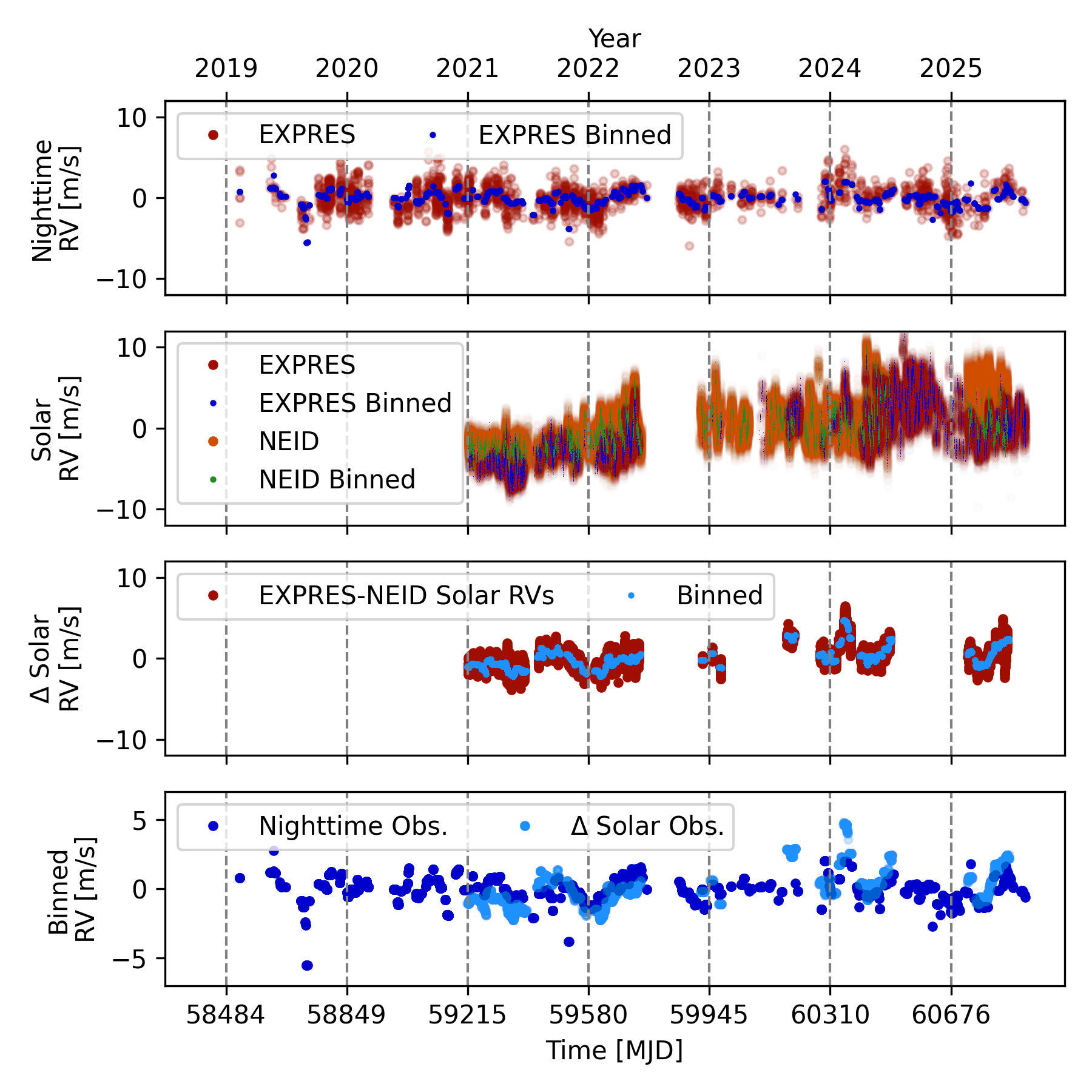
- How to read the axes and panels
- The stacked panels compare nighttime stellar RVs, two solar time series and their difference. The final panel uses a tighter velocity scale, so apparent amplitudes cannot be compared by visual height alone.
- What the plot is telling me
- Look for temporal agreement across the independent routes, especially the broad excursion around the highlighted interval. The agreement argues against a phenomenon belonging to only one observed star. It is the repeated timing, not a single conspicuous point, that gives the instrumental hypothesis weight.
- What it does not establish
- Smoothing alters which timescales remain visible. The solar difference can contain either instrument’s residuals; it is not a noiseless measurement of EXPRES drift.
Source Figure 1 and original caption ↗ · CC BY 4.0; author/source attribution retained. No data, axes or annotations have been redrawn.
What a comb-line bisector measures
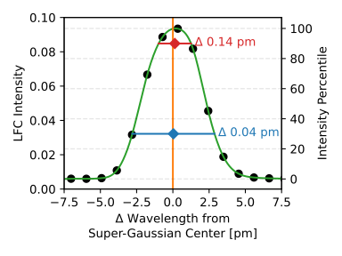
- How to read the axes and panels
- The horizontal direction describes position within a line profile; the markers sample the bisector at two intensity levels. A fitted centre and a bisector span are different observables.
- What the plot is telling me
- A symmetric profile can move without changing its span, while an asymmetric shape change can alter a measured centre. This picture explains why tracking line positions alone is incomplete. The span adds information about how the measurement kernel itself has changed.
- What it does not establish
- One illustrative line does not establish a universal profile model. Detector location, flux, blending and the chosen intensity levels can change the diagnostic’s sensitivity.
Source Figure 4 and original caption ↗ · CC BY 4.0; author/source attribution retained. No data, axes or annotations have been redrawn.
Telemetry beside optical-format diagnostics
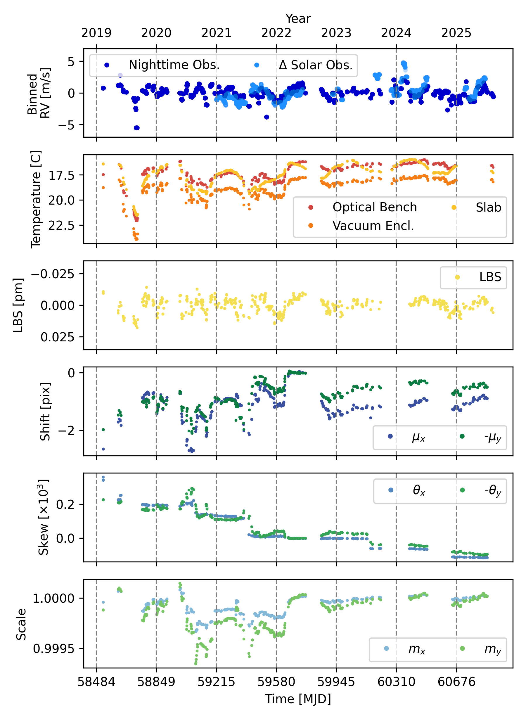
- How to read the axes and panels
- Time runs along the panels, while successive rows show different quantities with different units and scales. They should be compared in timing and shape, not by the apparent height of their fluctuations.
- What the plot is telling me
- The figure turns the vague idea of instrument health into several observable state variables. A disturbance can appear in temperature, asymmetry, shifts and scale factors differently. I would inspect which channels lead, lag or diverge during an intervention before choosing a more complicated regression.
- What it does not establish
- Visual correlation is not a causal ordering. Shared environmental forcing and correlated regressors can make several channels look persuasive without revealing which component caused the RV bias.
Source Figure 5 and original caption ↗ · CC BY 4.0; author/source attribution retained. No data, axes or annotations have been redrawn.
Building the correction in stages
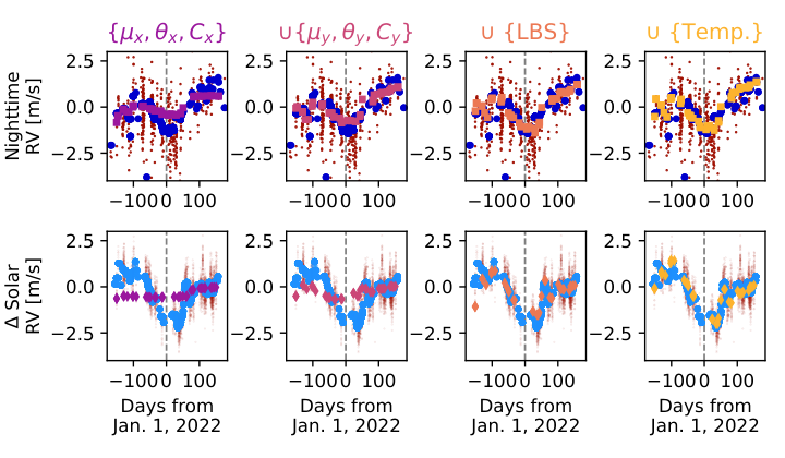
- How to read the axes and panels
- Columns add diagnostic groups cumulatively; the top and bottom rows use different observational routes. Each new column retains the preceding information.
- What the plot is telling me
- This is an ablation-style view of what each group contributes. The strongest interpretation is that geometric and profile information can supply structure missed by a temperature-only proxy. Compare the timing of the correction with the trend rather than rewarding any curve merely because it has more freedom.
- What it does not establish
- The sequence is not a ranking of independent physical causes. Correlated variables can redistribute explanatory power, and a smaller training residual need not imply better prediction.
Source Figure 7 and original caption ↗ · CC BY 4.0; author/source attribution retained. No data, axes or annotations have been redrawn.
Residual scatter as tracer groups are added
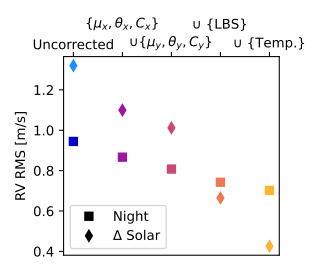
- How to read the axes and panels
- The horizontal axis represents cumulative model choices, not elapsed time. The vertical quantity is residual RMS for the binned series, with separate markers for the two data routes.
- What the plot is telling me
- A falling sequence shows that additional diagnostics explain variance under this evaluation. Read it together with the staged time series: a scalar improvement is easier to trust when it removes a coherent feature rather than just narrowing already random noise.
- What it does not establish
- RMS does not disclose whether a scientifically important period has been suppressed. The source also uses injections; this plot alone is not sufficient validation of a planet-search correction.
Source Figure 8 and original caption ↗ · CC BY 4.0; author/source attribution retained. No data, axes or annotations have been redrawn.
Injection–recovery and the false-period distribution
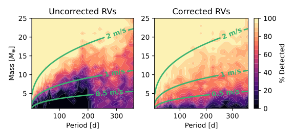
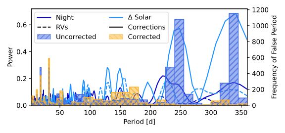
- How to read the axes and panels
- The upper maps compare recovery across injected mass and period before and after correction. The lower panels examine period-domain structure and the periods returned when recovery fails.
- What the plot is telling me
- The useful result is a change in recoverability over a region of parameter space, not a universal sensitivity multiplier. Compare the low-amplitude region and inspect whether instrumental-period concentrations diminish. The constant-amplitude curves help distinguish a mass boundary from a velocity-amplitude boundary.
- What it does not establish
- The adopted period-matching rule is stated in the original caption. It is not equivalent to a full discovery threshold or a guarantee that every orbit with a similar amplitude will be recovered.
Source Figure 10 and original caption ↗ · CC BY 4.0; author/source attribution retained. No data, axes or annotations have been redrawn.
Why ρ CrB is a frequency-domain demonstration
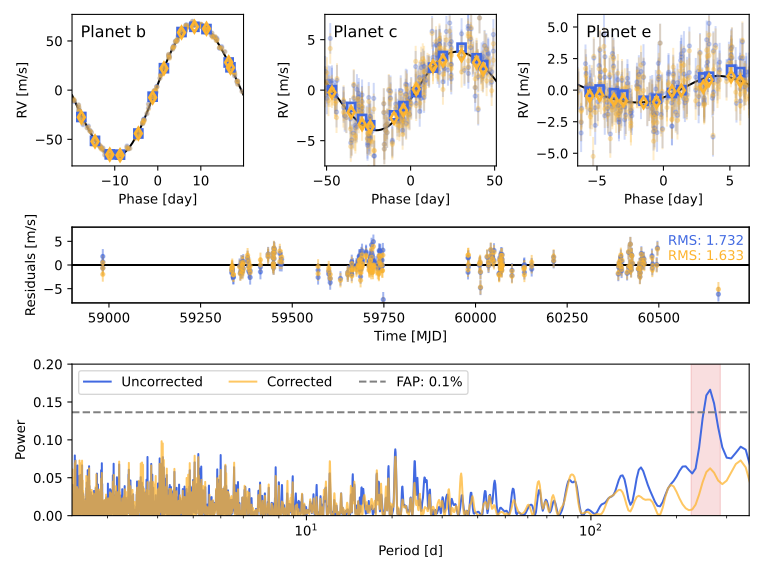
- How to read the axes and panels
- Phase-folded curves for the retained signals appear above periodograms of the three-planet residuals. The highlighted period range should be read against the earlier false-recovery exercise.
- What the plot is telling me
- This comparison makes a methodological point: two residual series can have rather similar scatter while differing substantially in coherent periodic structure. A disappearing residual peak can therefore matter more than a modest change in the headline RMS. Inspect whether the retained phase curves remain recognisable.
- What it does not establish
- This is evidence concerning the analysed observations and correction. It should not be restated as a general impossibility theorem for any additional planet in the system.
Source Figure 11 and original caption ↗ · CC BY 4.0; author/source attribution retained. No data, axes or annotations have been redrawn.
Sources and scope
- Zhao et al. (2026). Uncovering hidden systematics in extreme-precision radial velocity measurements. Read the version used: arXiv:2601.02296v1 · Abstract and version history.
This is a selective literature-reading note. Source claims appear in “What the authors report”; the comparison table, conceptual chain and proposed tests are analytical commentary. No new observations, reanalysis or experimental validation are claimed. Expanded source review: 21 October 2026.