Why this follows the ESPRESSO performance paper
The ESPRESSO performance paper establishes the instrument as a vacuum-stabilised, fibre-fed EPRV benchmark with resolving powers around R ≈ 140,000 and R ≈ 190,000 in 1-UT modes and a demonstrated RV precision better than 25 cm/s over one night.[2] Schmidt et al. then ask a narrower calibration question: once an advanced frequency comb is inserted into the system, what limits the wavelength solution?
This makes the paper a natural follow-up. ESPRESSO already has a strong instrument architecture. The EOM-comb test shows that calibration accuracy can still be limited by how the calibration light is delivered and modelled, especially through the calibration unit, fibre feeds, echellogram structure, and non-Gaussian line-spread function.
What the 34 GHz EOM comb is testing
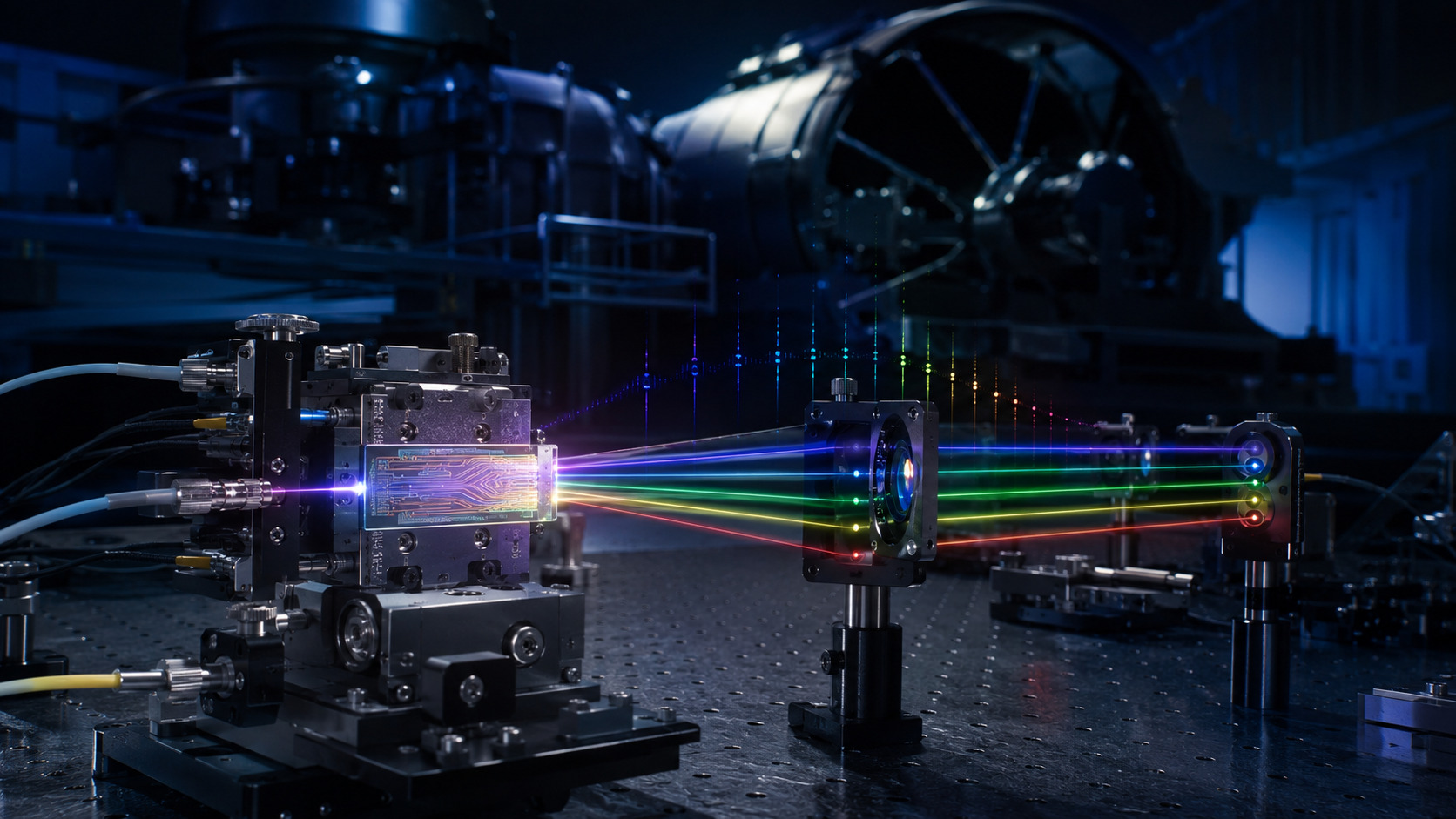
The paper tests a 34 GHz electro-optic modulation comb with ESPRESSO. The setup uses thin-film lithium-niobate waveguides for spectral broadening and harmonic generation, giving partial coverage of the infrared, visible and near-UV spectral ranges.[1]
The repetition spacing matters. Astronomical high-resolution spectrographs need comb modes that are separated enough to be resolved by the spectrograph, but dense enough to sample the wavelength solution. Earlier laser-comb discussions argued that mode spacings of roughly 5–30 GHz are typically needed for astronomical spectrographs; this 34 GHz implementation sits just above that practical range and is well matched to ESPRESSO-scale resolving power.[4]
| Quantity | Schmidt et al. result | Why it matters |
|---|---|---|
| Comb spacing | 34 GHz | Large enough for individual modes to be resolved by a high-resolution echelle spectrograph. |
| Technology | Electro-optic modulation with thin-film lithium-niobate waveguides | Compact route to broadening and harmonic generation across useful spectral regions. |
| Coverage | Partial IR, visible and near-UV coverage | Tests whether the source can support real spectrograph calibration, not only a narrow laboratory demonstration. |
| Key diagnostic | Background, line width, LSF and wavelength-solution comparison | Moves the test from “does the comb exist?” to “does it calibrate the delivered spectrum accurately?” |
Delivered spectra: background and line quality
The paper analyses spectrally diffuse background, line width and spectral quality of the delivered comb spectra. This is a useful emphasis because a comb spectrum is not automatically a clean wavelength ruler once it reaches the spectrograph. Background light, mode broadening, line asymmetry and detector sampling all affect how line centres are measured.
For a radial-velocity or wavelength-calibration pipeline, the relevant quantity is not only absolute frequency knowledge. It is the centre measured after the line passes through the instrument line-spread function and detector extraction. A source can have excellent metrological stability while still requiring careful modelling at the detector level.
Line-spread function: the model becomes part of the calibration
A central result is that excellent wavelength stability is only obtained when the non-Gaussian line-spread function is modelled accurately. This matches earlier ESPRESSO LSF work by Schmidt and Bouchy, which found that the ESPRESSO LSF is asymmetric, differs between slices and fibres, and varies along spectral orders. That work reduced discrepancies between independent wavelength solutions from about 50 m/s to around 10 m/s by using a more realistic LSF model.[3]
The message is important: the comb does not remove the need for a good instrument model. It reveals where the model is wrong. A pipeline that assumes an overly simple Gaussian line profile can turn a high-quality comb spectrum into a biased wavelength solution.
The 15 m/s discrepancy: source stability versus injection geometry
The strongest result is the comparison between the EOM comb and the ESPRESSO facility comb. Schmidt et al. find strong local discrepancies in wavelength calibration accuracy of up to 15 m/s, correlated with the echellogram structure.[1] The important interpretation is that these discrepancies do not originate from the lasers themselves. The authors attribute them to misalignments in the ESPRESSO calibration unit.
This is the main technical lesson of the paper. A laser frequency comb can be stable, but the delivered calibration can still be biased by how light enters the instrument. Calibration-unit alignment, fibre injection, near-field/far-field differences and slice illumination can create wavelength-solution structure that is not a property of the comb source.
Earlier ESPRESSO calibration work had already identified wavelength-dependent discrepancies up to 24 m/s when comparing the default ThAr/Fabry-Pérot solution to an independent LFC solution.[5] The new EOM-comb work makes the point sharper by showing that source comparison can diagnose local instrument-delivery effects.
Stability: 17 cm/s after appropriate modelling
Despite the local calibration-unit discrepancies, the paper demonstrates excellent stability of the wavelength calibration, with a scatter of only 17 cm/s.[1] The condition is important: this level is reached when the non-Gaussian line-spread function is modelled accurately.
This number should therefore be read carefully. It is not a simple “comb equals 17 cm/s” statement. It is a combined result of source quality, delivered spectrum, line-profile modelling, wavelength-solution method and instrument state. The stability sequence comprises 71 exposures over about 80 minutes; it is not a months-long on-sky RV test. The 17 cm/s value is the LFC-minus-FP drift residual for the second and third harmonics. The fainter fourth-harmonic region is instead near 60 cm/s, consistent with its photon noise.[1] That is why the paper is useful for reading after ESPRESSO: it shows how metrology and spectrograph optics meet in the actual data product.
Open technical questions after this reading
- Calibration-unit tolerance: What mechanical or optical tolerance on calibration-unit alignment is required to keep local wavelength errors below 10 cm/s rather than many m/s?
- Illumination monitoring: Can near-field and far-field monitoring of the calibration fibre detect the misalignment before it appears in the wavelength solution?
- Time dependence: Are the local 15 m/s discrepancies stable maps that can be corrected, or do they drift with temperature, alignment, fibre stress or calibration-unit usage?
- Transfer to science light: How closely does the calibration-light path reproduce the illumination state of the science fibres?
- LSF generalisation: Does the non-Gaussian LSF model remain valid across time, observing mode, fibre, slice and detector location?
- Operational complexity: Does the EOM-comb approach reduce long-term maintenance burden compared with facility comb systems, or does it move the complexity into data analysis and delivery diagnostics?
How I would test the delivery path
Proposed work, not performed: repeat controlled injection and reinjection cycles while holding source settings fixed. Compare wavelength-residual maps separately by order, fibre and slice rather than averaging them immediately into one offset.
I would then vary the flux envelope independently of the injection geometry and reduce the same frames with Gaussian and empirical LSF models. The comparison would test whether a centroid change follows the optical state, the line-profile model, or their interaction.
Finally, I would reserve a separate time sequence for validation. A model that fits one injection state should predict a withheld state before it is treated as an operational correction. The acceptance metric should include both wavelength-map bias and time-dependent scatter.
Calibration lesson for instrument-control work
The main lesson for smaller spectrograph projects is that calibration should be treated as a delivered optical state, not as a source specification. A stable source is necessary, but the calibration path must also be monitored. Fibre injection, illumination stability, line-profile modelling and detector extraction all enter the final wavelength solution.
This is useful when thinking about EXOhSPEC-style feedback work. A temperature loop can stabilise part of the instrument, but it does not replace calibration-path diagnostics. If the beam entering the spectrograph changes, or if the calibration and science paths are not equivalent, a thermally stable bench can still deliver a biased spectral format or wavelength solution.
Following the full technical argument
Follow the comb all the way from its clock to the detector
The reference frequency is only the beginning of the chain. Modulation, pulse preparation, nonlinear broadening, harmonic generation, coupling, mode scrambling and spectrograph injection each alter some property of the delivered light. Accurate tooth frequencies do not guarantee a flat envelope, negligible background or a perfectly stable illumination pattern.
A useful schematic comb law is νm = νseed + m frep. The spectrograph does not observe νm directly; it estimates a location from a sampled line convolved with an instrumental profile. This separates the metrology problem from the inverse problem. An error in the latter can remain even when the frequency reference is excellent.
The source comparison is unusually informative because independent comb systems interrogate the same instrument. Their disagreement should be localised by fibre, slice and order before it is summarised globally. A detector-wide mean can conceal the spatial structure that distinguishes a calibration-unit problem from a simple offset.
Background, intrinsic width and the empirical LSF
Diffuse flux beneath comb teeth changes the baseline from which line centres and wings are inferred. It is not merely a cosmetic loss of contrast. If that background or the flux envelope evolves, a mismatched profile model can turn an intensity change into an apparent displacement.
The observed line profile is a convolution of source and instrument, followed by detector sampling. A broader observed line is therefore not automatically a lower spectrograph resolving power; the intrinsic source width and fitting convention must be considered. The paper uses comparisons among calibration sources to separate parts of that problem.
The empirical LSF extends the model beyond a Gaussian width. Asymmetry, broad wings and position dependence matter when the desired displacement is a minute fraction of the line width. A log-flux view is useful because it exposes low-amplitude wings that a linear plot can hide. Those wings can influence a centroid even when they carry little total power.
Why stability and accuracy are allowed to disagree
A repeatable bias can leave a calibration stable in time while locally inaccurate. Conversely, a correct mean wavelength scale can still drift. The accuracy comparison and the short sequence therefore answer different questions, and their headline velocity units should not tempt the reader to compare them as the same metric.
The simultaneous FP provides a differential check on inferred drift. Agreement between slices is another internal consistency condition: adjacent slices should not acquire incompatible physical motions merely because their flux changes. The Gaussian-versus-empirical comparison is powerful because the raw observations are held fixed while the analysis model changes.
The short-sequence residual should remain attached to the bands, photon-noise level and observing duration actually tested. It does not establish multi-year science-RV performance. For future use I would demand transfer across injection cycles, source-envelope states and independent nights, with separate reporting of local wavelength bias and temporal repeatability.
Reading based on the full manuscript, including methods and discussion—not only its abstract. These explanations are original commentary; they are not a reproduced analysis or new experiment. Original manuscript · expanded 21 October 2026.
Paper plots, explained in detail
Read the paper plots alongside the explanations below. Each discussion keeps its source figure number and links to the original caption and context. Openly licensed panels are shown here; other figures open at the original paper. The explanations distinguish the plotted evidence from what it cannot establish.
The complete source and delivery architecture
- How to read the axes and panels
- The diagram follows modulation and frequency conversion through waveguide coupling and fibre delivery. Labels identify different physical operations, not interchangeable stability guarantees.
- What the plot is telling me
- Read it as a chain of potential transfer errors. Frequency referencing constrains the comb teeth, while alignment, power and modal behaviour can still change how the instrument sees them. That separation explains why the optical delivery system belongs in a calibration paper.
- What it does not establish
- A stable reference lock does not certify every downstream coupling state. The diagram is an architecture, not a measured tolerance budget.
Source Figure 1 and original caption ↗ · Original author/publisher rights retained. Open the figure at the source alongside this commentary; no additional copy is distributed here.
Diffuse background across the harmonics
- How to read the axes and panels
- The background-to-line measure varies with wavelength and filtering strategy. Marked harmonic centres organise the comparison.
- What the plot is telling me
- The plot asks whether a source with accurately known frequencies also supplies a clean spectrum to fit. Compare the wavelength dependence rather than choosing one appealing central value. A background change can interact with the model differently near the edge of a harmonic.
- What it does not establish
- This is not a direct wavelength-error axis. Translating background fraction into centroid error requires the profile, extraction and noise model.
Source Figure 7 and original caption ↗ · Original author/publisher rights retained. Open the figure at the source alongside this commentary; no additional copy is distributed here.
The non-Gaussian line-spread function
- How to read the axes and panels
- Profiles from positions within an order are offset for clarity and shown on a logarithmic flux scale, with Gaussian comparisons.
- What the plot is telling me
- The low-level wings and asymmetry are the important features. They explain why matching FWHM is not enough to make two line models equivalent. A model that looks adequate at the core can still misrepresent the structure relevant to very small shifts.
- What it does not establish
- Horizontal display offsets are not measured calibration offsets. Nor does one order establish a universal LSF for every fibre, slice, wavelength and future epoch.
Source Figure 10 and original caption ↗ · Original author/publisher rights retained. Open the figure at the source alongside this commentary; no additional copy is distributed here.
Local wavelength disagreement between independent combs
- How to read the axes and panels
- Velocity-equivalent residuals are organised across the spectral region, with fibres and slices distinguished. Measurements are aggregated over sub-order blocks.
- What the plot is telling me
- The structured pattern is the main result: a local mismatch tied to the instrument format is more diagnostic than a single global mean. Read the pattern alongside the discussion of injection geometry before blaming either frequency reference.
- What it does not establish
- The plotted values concern wavelength-solution accuracy in the comparison. They are not the random uncertainty of a stellar RV exposure or the drift residual of the later time sequence.
Source Figure 12 and original caption ↗ · Original author/publisher rights retained. Open the figure at the source alongside this commentary; no additional copy is distributed here.
An inadequate model can create incompatible slice drifts
- How to read the axes and panels
- The same exposure sequence is analysed with Gaussian profiles. Flux/background behaviour and inferred motions for the slices are displayed together.
- What the plot is telling me
- If nominally shared physical motion appears inconsistent between adjacent slices, that is a warning about the estimator. The correlation with intensity-related changes motivates a richer LSF/background treatment rather than accepting every fitted shift as real instrument motion.
- What it does not establish
- This is a controlled comparison of analysis assumptions, not evidence that the instrument physically develops the plotted differential slice displacement.
Source Figure 15 and original caption ↗ · Original author/publisher rights retained. Open the figure at the source alongside this commentary; no additional copy is distributed here.
The simultaneous-reference stability check
- How to read the axes and panels
- The panels separate spectral regions and compare slice-based LFC drifts with the FP reference, alongside changes in line and background flux.
- What the plot is telling me
- Read agreement of the differential motion and its residual scatter, not merely whether each curve is flat. Shared instrument drift can be present while the calibrators agree in tracking it. The source makes the wavelength-region and photon-noise qualifications important.
- What it does not establish
- A short, controlled sequence is not a multi-night or multi-year RV guarantee. The fainter short-wavelength region has a different noise level and should not inherit the best quoted residual.
Source Figure 16 and original caption ↗ · Original author/publisher rights retained. Open the figure at the source alongside this commentary; no additional copy is distributed here.
References
- T. M. Schmidt et al. (2026), Test of a 34 GHz EOM laser frequency comb at ESPRESSO, accepted for publication in MNRAS; arXiv:2603.17908v1, full text.
- F. Pepe et al. (2021), ESPRESSO@VLT: On-sky performance and first results, Astronomy & Astrophysics 645, A96; arXiv:2010.00316.
- T. M. Schmidt and F. Bouchy (2024), Characterization of the ESPRESSO line-spread function and improvement of the wavelength calibration accuracy, arXiv:2404.05283.
- M. T. Murphy et al. (2007), High-precision wavelength calibration of astronomical spectrographs with laser frequency combs, arXiv:astro-ph/0703622.
- T. M. Schmidt et al. (2020), Fundamental physics with ESPRESSO: towards an accurate wavelength calibration for a precision test of the fine-structure constant, arXiv:2011.13963.