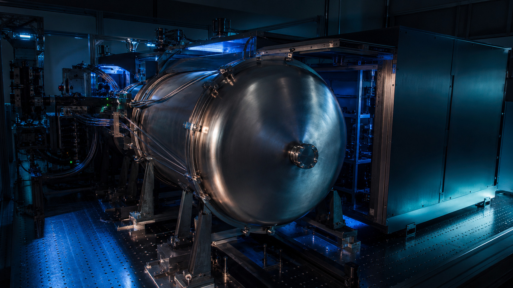
What ESPRESSO is designed to solve
ESPRESSO is the Echelle SPectrograph for Rocky Exoplanets and Stable Spectroscopic Observations. In 1-UT High Resolution mode, the paper reports resolving power around R ≈ 140,000 over 378.2–788.7 nm; the Ultra High Resolution mode reaches approximately R ≈ 190,000; and the 4-UT mode provides an equivalent 16 m aperture at approximately R ≈ 70,000.[1]
The performance numbers define the engineering problem. The paper reports throughput above 10% near 550 nm under nominal 0.65 arcsec seeing, radial-velocity precision better than 25 cm/s over one night, and better than 50 cm/s over several months. These values are described as limited by photon noise and stellar jitter, consistent with a 10 cm/s instrumental precision floor.[1]
| Quantity | Reported value | Why it matters here |
|---|---|---|
| 1-UT HR / UHR resolution | R ≈ 140,000 / 190,000 | Benchmark scale for high-resolution optical EPRV hardware. |
| 4-UT mode | Equivalent 16 m aperture, R ≈ 70,000 | Combines collecting area with additional optical-delivery constraints. |
| Wavelength range | 378.2–788.7 nm | Broad visible coverage increases calibration, detector, blaze and order-level systematics. |
| Throughput | >10% near 550 nm | Directly controls the photon-noise-limited RV floor. |
Coudé train: the instrument begins before the bench
ESPRESSO receives light from the VLT Unit Telescopes through the Coudé train before the beam reaches the Combined Coudé Laboratory. The front-end module includes atmospheric-dispersion correction, field and pupil stabilisation, and calibration-light injection. The telescope-to-lab optical path is therefore part of the instrument, not merely delivery hardware.
This matters because detector motion or wavelength drift cannot automatically be assigned to the bench. It may originate in input illumination, pupil motion, fibre injection, calibration geometry, pressure and temperature changes, or a coupled combination of these effects.
Fibre feed, pseudo-slit, and scrambling
The fibre feed uses octagonal fibres and a double scrambler. The paper describes the scrambler as exchanging near-field and far-field illumination so guiding residuals and pupil wobble are suppressed before they become spectral-format changes. A stable wavelength solution is not sufficient if the light enters the spectrograph in a different spatial state from exposure to exposure.
The pseudo-slit and spectral-format figures make this visible. HR, UHR and MR modes map fibre outputs differently onto the detector. Residual near-field or far-field variation can alter line shapes, extraction weights or order-dependent centroids.
Vacuum and multi-shell thermal stability
ESPRESSO is placed inside a large vacuum vessel in the Combined Coudé Laboratory. The vacuum removes air-column refractive-index variations from the optical path, while multiple actively controlled thermal shells reduce the disturbance that reaches the optical bench. This is a cascade, not a single-loop control strategy.
The missing piece, from a control-analysis point of view, is the frequency-domain response. An RMS temperature number does not show whether remaining thermal power lives on exposure timescales, nightly timescales or seasonal timescales.
Resolving power is not a single number
The resolving-power maps are more useful than a headline R value because they show dependence on observing mode, detector position, order, slice and wavelength. For precision work, resolution should be treated as a mapped quantity across the extracted format, not as one scalar label.
Throughput and efficiency: high resolution is not free
The efficiency plots show that throughput cannot be separated from resolution and seeing. HR mode reaches more than 10% photon-detection efficiency near 550 nm, while the blue end drops substantially. UHR mode increases resolving power but makes aperture, seeing, slit loss and fibre size more restrictive. The design trade-off is therefore not “higher resolving power is always better”.
If a design chases resolution without tracking throughput, radial-velocity precision can worsen because photon noise grows faster than information content improves. Resolution, throughput, fibre diameter, seeing, detector efficiency and target type belong in the same error budget.
RV precision: short-term and long-term validation
The internal precision versus S/N plot links photon noise, spectral type and information content. The seven-hour HD 85512 time series reports approximately 28 cm/s RMS for single 300 s exposures, close to the 25 cm/s photon-noise estimate, and binning five points reduces the scatter to roughly 8 cm/s.[1]
The long-baseline τ Ceti plots show the operational reality. The paper distinguishes data before and after the June 2019 fibre upgrade, with raw scatter changing from around 0.94 m/s before the intervention to around 0.72 m/s after it, and nightly-binned post-upgrade scatter around 0.58 m/s.[1] Short-term precision and long-baseline repeatability are not the same performance claim.
Calibration strategy: ThAr, Fabry-Pérot, and the LFC boundary
ThAr lamps provide absolute wavelength anchors, while a white-light Fabry-Pérot etalon provides dense drift monitoring. The laser-frequency comb was intended to provide a more complete calibration reference, but at the time of the performance paper it was not yet fully reliable or routine.[1]
Later calibration papers sharpen this section. Schmidt et al. tested a 34 GHz EOM comb at ESPRESSO and found that the source itself was stable, while calibration-unit injection geometry could introduce local wavelength-solution systematics.[2] Kreider et al. showed that Fabry-Pérot resonators can drift chromatically, which means an FP grid cannot always be treated as a rigid ruler.[3]
Open technical questions after this reading
- Thermal transfer function: What is the frequency-domain transfer function from room to shell, vessel, bench and wavelength solution?
- Fibre-link root cause: The paper reports a fibre-link throughput deficiency that required repair. Was the dominant issue alignment, coating degradation, stress, modal behaviour, or another mechanism?
- Calibration injection repeatability: If later comb tests reveal calibration-unit injection systematics, what tolerance should be assigned to the fibre-head or switching mechanism?
- Scrambling residuals: What residual near-field or pupil variation remains at the pseudo-slit under different seeing and guiding conditions?
- 4-UT stability: Has the 4-UT mode been demonstrated over the same long-baseline RV stability window as the 1-UT mode?
Connection to EXOhSPEC
This paper gives a checklist rather than a recipe. For EXOhSPEC, the writing should state where the disturbance enters, what each control or shielding layer attenuates, and which measured optical quantity proves that the correction is working. Temperature stability alone is not the final metric; the final metric is whether the optical path, spectral format, centroid, or wavelength solution becomes more stable.
The same point changes how TEC feedback should be presented. A TEC loop should appear as one element of a stability architecture: environmental sensing, thermal actuation, optical-path monitoring, image or echellogram tracking, calibration diagnostics, and a quantified residual error budget.
Following the full technical argument
Extraction, observing modes and the information preserved in the data
The instrument description is not complete at the vacuum vessel. Acquisition, guiding, the sliced fibre images, detector sampling and the reduction chain determine which information survives into a spectrum. The raw-format figure makes that connection tangible: calibration and science traces have a specific geometry that a pipeline must model consistently.
Observing modes trade collecting area, resolving power, sampling and sensitivity. These are not cosmetic settings. A binning choice changes read-noise and sampling behaviour, while a different fibre aperture changes the seeing-dependent throughput. Comparing modes fairly requires a common science objective and an explicit exposure-time or precision metric.
A reduced spectrum should also be read as a measurement carrying atmospheric structure and processing choices. The blue and red examples contain different information and different potential contaminants. Wide wavelength coverage increases scientific leverage, but also expands the burden of throughput characterisation, wavelength calibration and telluric treatment.
Performance is a family of experiments, not one record number
The source supplies several complementary tests: resolution maps, efficiency versus wavelength and seeing, S/N versus magnitude, internal RV uncertainty, time-domain repeatability and telescope-path equivalence. Each controls a different part of the error budget. No single plot replaces the others.
The upper envelope of an S/N–magnitude relation describes favourable observing conditions rather than a guarantee for every exposure. Likewise, an internal photon-noise estimate concerns information in a measured spectrum, not the full uncertainty after stellar variability, interventions and calibration systematics are included. Distinguishing these definitions prevents an impressive number from acquiring a broader meaning than the experiment supports.
Interventions need explicit treatment. An improvement in throughput after a fibre change is scientifically valuable, but combining the time series without considering offsets or changed instrument response could confuse an RV analysis. A commissioning paper is most useful when it records those operational details rather than presenting a single unbroken idealised instrument.
The science cases explain why the engineering trade-offs matter
The guaranteed-time programme connects the design to more than one kind of measurement. A high-S/N bright-star spectrum and a faint quasar spectrum place different demands on resolution, collecting area and calibration fidelity. The science examples should therefore be read as demonstrations of distinct capabilities rather than as one universal observing recipe.
For a planet-search example, phase-folded RV agreement checks a repeatable signal, while binning and high-cadence observations probe the residual noise and stellar variability. A clean folded curve does not imply that the unmodelled time series is white noise. That is why the adjacent binning and p-mode figures deserve their own reading.
For absorption-line science, stable spectral structure and accurate local wavelength information can matter differently from a star’s global Doppler shift. The quasar examples broaden the calibration lesson: a wavelength distortion that partly averages out in one estimator may remain important in another. The instrument has to be characterised for the observable actually being inferred.
Reading based on the full manuscript, including methods and discussion—not only its abstract. These explanations are original commentary; they are not a reproduced analysis or new experiment. Original manuscript · expanded 21 October 2026.
Figure-by-figure reading
The figure panels below anchor the discussion to specific instrument-design and performance figures from Pepe et al. They are included where they clarify architecture, spectral format, resolving power, throughput, radial-velocity precision, and telescope-path equivalence.
Further source figures: reduction, sensitivity and science cases
Read the paper plots alongside the explanations below. Each discussion keeps its source figure number and links to the original caption and context. Openly licensed panels are shown here; other figures open at the original paper. The explanations distinguish the plotted evidence from what it cannot establish.
The science and calibration traces in a raw frame
- How to read the axes and panels
- This is a detector-space view with the dispersion orientation stated in the source. Stellar and Fabry–Pérot traces appear in the sliced spectral format.
- What the plot is telling me
- Use it to connect the abstract pseudo-slit diagram with actual recorded information. Extraction is not just summing a bright line: the pipeline must identify traces, model their profiles and keep nearby information distinct.
- What it does not establish
- A raw display is not a calibrated wavelength solution. Visual separation of traces does not establish negligible cross-talk or an unbiased extraction.
Source Figure 7 and original caption ↗ · Original author/publisher rights retained. Open the figure at the source alongside this commentary; no additional copy is distributed here.
A broad spectrum and two very different spectral regions
- How to read the axes and panels
- The panels show an extracted spectrum and selected blue/red regions, making wavelength-dependent structure visible.
- What the plot is telling me
- The spectrum demonstrates that broad coverage brings diverse information into one instrument. Read the atmospheric absorption in its own role: a sharp feature is not automatically a stellar feature or an equally useful RV constraint. Different regions need different masks and calibration checks.
- What it does not establish
- A plotted example is not a sensitivity guarantee at every wavelength or target magnitude. The plotted processing and observing mode remain part of the measurement.
Source Figure 10 and original caption ↗ · Original author/publisher rights retained. Open the figure at the source alongside this commentary; no additional copy is distributed here.
The fibre intervention and seeing-dependent efficiency
- How to read the axes and panels
- Efficiency near the stated wavelength is compared with image quality before and after the upgrade.
- What the plot is telling me
- The comparison connects an engineering intervention to photon delivery, rather than assuming throughput from the optical design alone. Inspect both the separation of the populations and their dependence on seeing. The gain should be understood under comparable conditions.
- What it does not establish
- A before/after efficiency plot does not by itself isolate every physical cause or establish the RV zero-point stability of the new configuration.
Source Figure 12 and original caption ↗ · Original author/publisher rights retained. Open the figure at the source alongside this commentary; no additional copy is distributed here.
S/N versus magnitude is not a single exposure promise
- How to read the axes and panels
- Target magnitude is compared with measured S/N after normalising exposure duration, and an envelope indicates favourable conditions.
- What the plot is telling me
- The population below the envelope is informative: observing conditions and throughput variation are operational realities. A planning calculation should therefore distinguish an achievable envelope from a typical result and a conservative exposure estimate.
- What it does not establish
- Exposure normalisation does not make all observations otherwise identical. Seeing, airmass, source spectrum and instrumental state can still differ.
Source Figure 16 and original caption ↗ · Original author/publisher rights retained. Open the figure at the source alongside this commentary; no additional copy is distributed here.
The faint-source quasar demonstration
- How to read the axes and panels
- The reduced quasar spectrum includes emission and absorption structure on the plotted wavelength grid.
- What the plot is telling me
- This example tests a different part of the instrument’s usefulness from bright-star RV work. Collecting area, extraction, sampling and calibration must produce a scientifically usable faint spectrum, not merely an appealing detector image.
- What it does not establish
- A successful example does not establish completeness of a survey or uniquely identify every absorption feature. Resampling also affects how neighbouring errors should be interpreted.
Source Figure 19 and original caption ↗ · Original author/publisher rights retained. Open the figure at the source alongside this commentary; no additional copy is distributed here.
A known periodic RV signal as an observing demonstration
- How to read the axes and panels
- The phase-folded velocities compare ESPRESSO with an established data set for a known short-period signal.
- What the plot is telling me
- The relevant reading is whether the measurements recover a coherent orbital variation on a compatible velocity scale. Phase folding is useful for that narrow check because it aligns repeated orbital phases.
- What it does not establish
- Folding discards temporal ordering. It cannot by itself show that instrument drift, evolving stellar activity or sampling aliases are absent from the original time series.
Source Figure 25 and original caption ↗ · Original author/publisher rights retained. Open the figure at the source alongside this commentary; no additional copy is distributed here.
Does averaging behave like independent noise?
- How to read the axes and panels
- Residual dispersion is plotted against the amount of binning rather than against observing date.
- What the plot is telling me
- For independent, similarly weighted measurements the standard-error expectation scales approximately as N⁻¹ᐟ². Departures motivate inspection of correlation, stellar variability and unequal sampling. This makes the plot an error-model diagnostic, not merely a route to a smaller reported scatter.
- What it does not establish
- Binning changes time resolution and the signal one can recover. A small binned scatter does not establish the same precision for individual exposures or for all timescales.
Source Figure 26 and original caption ↗ · Original author/publisher rights retained. Open the figure at the source alongside this commentary; no additional copy is distributed here.
Short-timescale stellar variability remains visible
- How to read the axes and panels
- The high-cadence RV sequence resolves changes within one observing window.
- What the plot is telling me
- The oscillatory structure illustrates why an ultra-stable spectrograph does not make a star a constant reference. Exposure duration and cadence can average or resolve stellar modes differently, so the observing strategy belongs in the precision budget.
- What it does not establish
- A short sequence cannot establish the long-term stellar or instrumental noise model. Its visible structure should not all be assigned to hardware drift.
Source Figure 27 and original caption ↗ · Original author/publisher rights retained. Open the figure at the source alongside this commentary; no additional copy is distributed here.
Different absorption systems probe different sight lines
- How to read the axes and panels
- Two sight lines through a lensed quasar are compared in selected absorption regions, with separate panels for different spectral structures.
- What the plot is telling me
- The comparison shows that high-fidelity spectra can test spatially different material along closely related lines of sight. Relative profile structure is the observable; simply quoting a global RV precision would not describe this experiment adequately.
- What it does not establish
- A difference in an absorption profile requires line identification and astrophysical interpretation. A visual comparison alone does not uniquely determine the absorbing gas geometry or separate every calibration contribution.
Source Figure 28 and original caption ↗ · Original author/publisher rights retained. Open the figure at the source alongside this commentary; no additional copy is distributed here.
References
- F. Pepe et al. (2021), ESPRESSO@VLT: On-sky performance and first results, Astronomy & Astrophysics 645, A96; arXiv:2010.00316.
- T. M. Schmidt et al. (2026), Test of a 34 GHz EOM laser frequency comb at ESPRESSO, arXiv:2603.17908.
- M. K. Kreider et al. (2025), Quantifying broadband chromatic drifts in Fabry-Pérot resonators for exoplanet science, Nature Astronomy / arXiv:2210.10988.