What the authors report
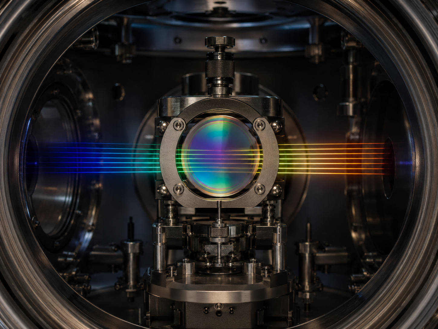
Kreider et al. compare Fabry–Pérot modes with laser frequency combs in HPF and NEID, tracking up to about 13,000 modes. Wavelength-dependent drift is modelled through changes in dielectric mirror layers in addition to a bulk cavity term. The preprint reports frequency-drift precision approaching 10⁻¹¹ per day, equivalent to about 3 mm/s per day. That is a precision on drift behaviour—not a demonstrated 3 mm/s on-sky stellar RV floor. [1]
Reading the evidence
| Model component | Conceptual signature | Diagnostic risk |
|---|---|---|
| Bulk optical length | A shared fractional-frequency component. | Can hide wavelength-dependent residuals if used alone. |
| Mirror reflection phase | A wavelength-dependent contribution. | A narrow reference cannot determine its full shape. |
| Instrument and extraction | A detector-dependent contribution. | May be confused with calibrator drift without independent comparison. |
The measurement chain
A conceptual reading aid, not measured data or a reproduction of a paper figure:
- Cavity and coating changes
- Wavelength-dependent modes
- Independent reference comparison
- Validated calibration residual
The resonance includes the mirrors
A useful schematic resonance condition is 2knL + φ₁ + φ₂ = 2πm, where k is vacuum wavenumber and φ₁, φ₂ are reflection phases. If the reflection phases vary with wavelength and change with time, the mode grid need not drift as a rigid scale. This simplified expression explains why a cavity-length-only model can be incomplete.
The distinction is between stabilising a physical assembly and stabilising every optical resonance it produces. A sensor or reference that strongly constrains one degree of freedom may leave another unobserved. A lock at one wavelength therefore needs broadband validation before its correction is extrapolated.
Separating the ruler from the instrument
A calibrator is measured through the same instrument whose drift it is meant to diagnose. That creates an identifiability problem: detector motion, illumination changes and a moving reference can produce superficially similar residuals. An independent frequency reference helps break that ambiguity, but only over the region and cadence actually sampled.
I would retain wavelength-resolved residual maps throughout the analysis. A weighted mean is useful for operational monitoring, yet opposite-sign errors in different spectral regions may cancel in that mean while still biasing a star with different line weights.
Why a physical fit still needs validation
A plausible coating model need not uniquely identify which microscopic material process occurred. Thickness and refractive-index perturbations can have correlated signatures. I would report the model’s explanatory power separately from any claim of a uniquely recovered physical mechanism.
Extrapolation is another boundary. A fit over one time interval is not automatically a forecast through maintenance, a temperature cycle or a change in illumination. The reference cadence should be justified by prediction error, not simply by an attractive average drift rate.
How I would test an FP calibration strategy
Wavelength holdout: fit on separated wavelength regions and predict modes not used in the fit. Compare a bulk-only model with a modest chromatic model under the same validation scheme.
Time holdout: forecast the next reference interval and record the full residual distribution. Refit only after evaluating that forecast; otherwise model flexibility can disguise poor predictive performance.
Science weighting: propagate the residual map through representative stellar line weights. A broadband mean and a cool-star RV estimator need not have the same sensitivity to chromatic error.
A practical calibration lesson
For an EXOhSPEC-style stability budget, I would keep calibrator ageing separate from the spectrograph’s thermal response. The two can share timescales while requiring different interventions.
The operational product should include an evolving wavelength-dependent calibration residual and its uncertainty. That is more informative than a single reassuring offset, and gives a concrete criterion for when an independent absolute reference is needed.
Following the full technical argument
The central inference is differential and broadband
The experiment does not treat the spectrograph as an immutable detector of an etalon. It compares etalon resonances against a frequency-comb reference across the band. Changes common to both can be distinguished from changes of the etalon relative to that reference. The spectral coverage is crucial because one reference wavelength cannot reveal how distant modes separate.
For a simple cavity, increasing optical length lowers the resonant frequency at fixed mode number. This yields a comparatively simple fractional-frequency pattern. Once the mirrors contribute a wavelength-dependent reflection phase, the same intuitive rigid-ruler picture is no longer complete. Opposite trends at different wavelengths need not mean the physical spacer simultaneously grows and shrinks.
That distinction also sets an operational requirement. A densely populated calibrator can provide excellent interpolation while still carrying an evolving reference error. The density of its lines and their absolute long-term stability are independent properties. Both must appear in a calibration budget.
Why coating structure is an explanatory model, not just a flexible curve
A multilayer mirror is designed through interference among reflected amplitudes. Its reflectivity and reflection phase depend on layer thicknesses and refractive indices. Small material changes can therefore reshape the frequency response even when a mechanical spacer is extremely stable.
The paper’s perturbative comparison asks which layer changes produce the observed wavelength pattern. This is more constrained than fitting an arbitrary polynomial to drift. The shape, sign changes and relative spectral behaviour become evidence about where a perturbation could reside. A successful model should explain those features rather than merely reproduce the mean rate.
However, fitting thickness and refractive-index changes does not uniquely identify their microscopic cause. Stress relaxation and a surface alteration can have related effective optical consequences. The uncertainty in the manufactured coating structure also matters. I would separate three claims: chromatic drift is observed; certain coating perturbations explain its structure; the exact underlying ageing mechanism still needs dedicated material evidence.
How to read alternatives, residuals and long-baseline implications
A competing mechanism should be compared in shape as well as amplitude. A temperature or alignment perturbation large enough to match the overall scale can still predict the wrong wavelength dependence. The alternative-mechanism figure is therefore part of the argument, not an incidental appendix.
Residuals identify what the physical model has not explained. Smooth structure may indicate an incomplete layer model or imperfect knowledge of the as-built coating. Treating every residual as independent noise would exaggerate confidence in extrapolating the correction to new times or wavelengths.
For a survey, the practical question is how accurately an etalon can predict its own future grid between independent reference observations. That requires held-out temporal validation and science-weighted residuals. This paper motivates a better calibration architecture, but it does not remove stellar variability, detector effects or the need for an end-to-end RV error budget.
Reading based on the full manuscript, including methods and discussion—not only its abstract. These explanations are original commentary; they are not a reproduced analysis or new experiment. Original manuscript · expanded 21 October 2026.
Paper plots, explained in detail
Read the paper plots alongside the explanations below. Each discussion keeps its source figure number and links to the original caption and context. Openly licensed panels are shown here; other figures open at the original paper. The explanations distinguish the plotted evidence from what it cannot establish.
How the relative drift is measured
- How to read the axes and panels
- The panels progress from Doppler spectroscopy to the calibration arrangement and finally the spectral dependence of drift. Distinguish the illustrative setup panels from measured or derived trend quantities.
- What the plot is telling me
- The key operation is subtracting the stable-reference behaviour from the etalon behaviour. That gives a way to ask whether the ruler changes independently of the spectrograph. The final wavelength-dependent picture explains why one scalar drift correction can be inadequate.
- What it does not establish
- A schematic of differential measurement does not imply that every instrumental systematic cancels perfectly. Illumination and extraction differences still require control.
Source Figure 1 and original caption ↗ · Original author/publisher rights retained. Open the figure at the source alongside this commentary; no additional copy is distributed here.
Spacer motion and coating perturbations make different patterns
- How to read the axes and panels
- The panels compare a simple length change with changes in mirror structures and selected layers. Wavelength is the organising axis of the calculated responses.
- What the plot is telling me
- A bulk perturbation produces a much simpler fractional pattern than some coating changes. The oscillatory response of a complex stack provides a discriminating signature: the shape can constrain a model even when several mechanisms produce similar average amplitudes.
- What it does not establish
- These are model responses to specified perturbations, not direct imaging of layers ageing. Their interpretation depends on the assumed stack and material properties.
Source Figure 2 and original caption ↗ · Original author/publisher rights retained. Open the figure at the source alongside this commentary; no additional copy is distributed here.
The physical model confronted with the measurements
- How to read the axes and panels
- The figure places fitted drift behaviour above residual panels for the two etalons. The parameter tables should be read together with the residual curves, not separately.
- What the plot is telling me
- A useful fit follows the wavelength structure and leaves a physically plausible parameter combination. Compare what the additional layer freedom changes in the residuals. If broad patterns remain, a small overall RMS does not mean the model has captured every relevant degree of freedom.
- What it does not establish
- An improved fit is not unique proof of a microscopic relaxation process. Correlations between parameters and uncertainty in the as-built mirror remain part of the interpretation.
Source Figure 3 and original caption ↗ · Original author/publisher rights retained. Open the figure at the source alongside this commentary; no additional copy is distributed here.
Testing alternative mechanisms by their spectral signatures
- How to read the axes and panels
- The panels show calculated effects of incidence angle, polarisation-related changes and a uniform thermal perturbation. Each is a specific alternative with stated assumptions.
- What the plot is telling me
- The comparison illustrates why matching a number is weaker than matching a spectral pattern. An alternative can produce a sizeable shift while failing to reproduce the observed oscillation structure. Shape disagreement is therefore informative physical evidence.
- What it does not establish
- These calculations constrain the tested scenarios. They do not exclude every possible spatial temperature gradient, complex contamination process or combined disturbance in a different instrument.
Source Figure 4 and original caption ↗ · Original author/publisher rights retained. Open the figure at the source alongside this commentary; no additional copy is distributed here.
Sources and scope
- Kreider et al. (2025). Quantifying broadband chromatic drifts in Fabry–Pérot resonators for exoplanet science. Read the version used: arXiv:2210.10988v2 · Abstract and version history.
- Publisher record: Nature Astronomy (2025), DOI 10.1038/s41550-025-02486-x.
This is a selective literature-reading note. Source claims appear in “What the authors report”; the comparison table, conceptual chain and proposed tests are analytical commentary. No new observations, reanalysis or experimental validation are claimed. Expanded source review: 21 October 2026.