This note describes the control model used in the V6b design for EXOhSPEC stability experiments. It separates the scientific logic from laboratory-specific hardware interfaces, serial ports and run configuration.
The control hierarchy is TEC-primary with active-optics fine trim:
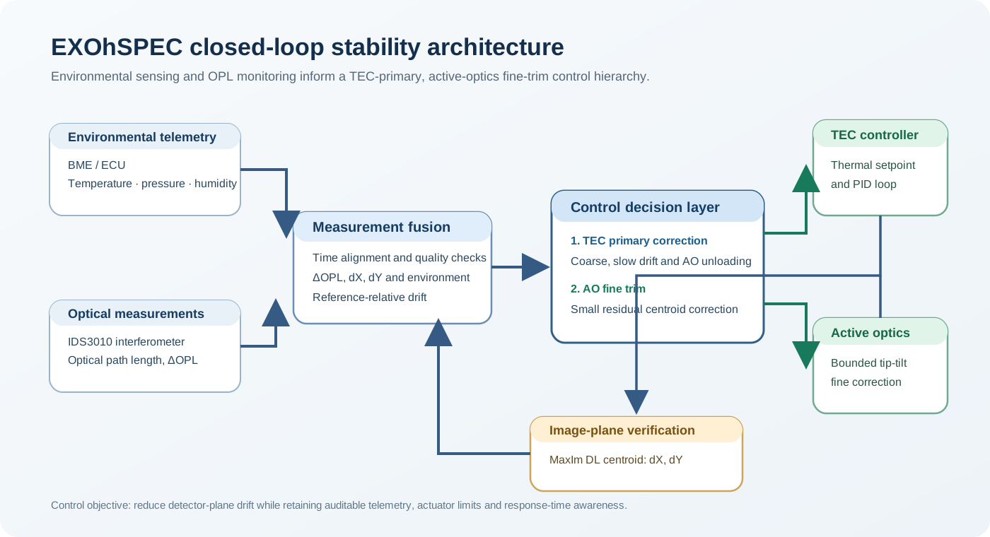
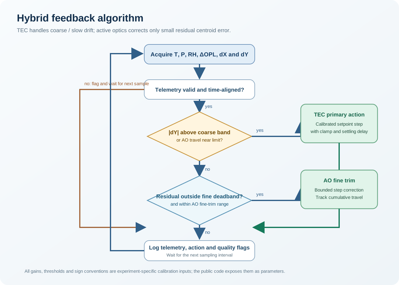
The architecture is shown in ../figures/exohspec_feedback_architecture.svg, and the decision sequence in ../figures/hybrid_feedback_algorithm.svg.
At sample index $k$, the controller forms a synchronised measurement vector:
\[\mathbf{z}_k = \begin{bmatrix} \Delta x_k & \Delta y_k & L_k & T_{\mathrm{in},k} & H_{\mathrm{in},k} & P_{\mathrm{in},k} & T_{\mathrm{out},k} & H_{\mathrm{out},k} & P_{\mathrm{out},k} \end{bmatrix}^{\mathsf{T}}.\]Here, $\Delta x$ and $\Delta y$ are centroid offsets from the current reference, and $L$ is optical path length (OPL).
The radial image-plane error used for reporting is:
\[r_k = \sqrt{\Delta x_k^2 + \Delta y_k^2}.\]The controller also evaluates short-window rates:
\[\dot{T}_{\mathrm{in},k} \approx \frac{T_{\mathrm{in},k}-T_{\mathrm{in},k-m}}{t_k-t_{k-m}}, \qquad \dot{T}_{\mathrm{out},k} \approx \frac{T_{\mathrm{out},k}-T_{\mathrm{out},k-m}}{t_k-t_{k-m}}, \qquad \dot{L}_k \approx \frac{L_k-L_{k-m}}{t_k-t_{k-m}}.\]The V6b controller calculates a temperature-, pressure- and humidity-dependent refractive-index proxy:
\[n_{\mathrm{proxy}}(T,P,H;\lambda) = 1 + \frac{\alpha(\lambda)P}{RT} - \frac{\beta e(T,H)}{RT}.\]Here, $e(T,H)$ is the water-vapour partial pressure estimated from temperature and relative humidity. This quantity is used as an environmental predictor and trend indicator. It is not presented here as a substitute for a metrology-standard air-index calculation; the publication analysis should state the exact adopted refractivity formulation and its valid pressure, temperature and wavelength range.
The controller begins with an open-loop warm-up period. Its purpose is to establish a stable centroid reference and estimate run-specific behaviour before actuation starts.
The key principle is that the environmental response is identified per run, rather than assumed to be constant across all experiments. A fixed coefficient may be inaccurate when the thermal state, HVAC conditions, optical alignment or actuator history differ from the calibration run.
For a feedback run, the empirical thermal OPL gain is:
\[g_T = \frac{\partial L}{\partial T_{\mathrm{set}}}.\]The active-optics image-plane calibration is represented by:
\[\begin{bmatrix} \Delta x \\ \Delta y \end{bmatrix} = \mathbf{M}_{\mathrm{AO}} \begin{bmatrix} s_x \\ s_y \end{bmatrix}.\]Here, $s_x$ and $s_y$ are commanded AO steps and $\mathbf{M}_{\mathrm{AO}}$ is measured from a dedicated calibration sequence.
The V6b design fits a rolling ordinary-least-squares model using the recent control history:
\[\widehat{\Delta T}_{\mathrm{OLS},k} = b_0 + b_L\Delta L_k + b_n\left(10^6\Delta n_{\mathrm{proxy},k}\right) + b_H\Delta H_k + b_P\Delta P_k + b_{\dot{T}}\dot{T}_{\mathrm{in},k}.\]Only a model that reaches a pre-defined minimum sample count and goodness-of-fit threshold is used. Otherwise, the controller falls back to centroid-error feedback.
A physically motivated OPL feed-forward term is:
\[\Delta T_{\mathrm{ff},k} = -\frac{\Delta L_k}{g_T}.\]The model and feed-forward estimates are blended and bounded:
\[\Delta T_{\mathrm{cmd},k} = \operatorname{sat}_{\pm\Delta T_{\max}} \left[(1-w)\widehat{\Delta T}_{\mathrm{OLS},k} + w\Delta T_{\mathrm{ff},k}\right].\]When the rolling model is unavailable or rejected, the fallback PI law is:
\[I_k = \operatorname{clip}(I_{k-1}+\Delta y_k, -I_{\max}, I_{\max}),\] \[\Delta T_{\mathrm{PI},k} = -\left(K_P\Delta y_k + K_I I_k\right),\]followed by the same thermal-step saturation.
| The TEC update interval is shortened when $ | \dot{L} | $ or $ | \dot{T}_{\mathrm{in}} | $ is elevated, and lengthened in a quiet state. A pre-emptive trigger estimates whether OPL motion is likely to move the image outside the coarse-control region before the next scheduled thermal update: |
where $S_{L\rightarrow y}$ is the empirical OPL-to-pixel sensitivity.
Rapid external-temperature motion is treated as an HVAC transient. The controller can defer a non-urgent thermal command during such a transient to avoid reacting to a disturbance that may reverse on the next sample.
Let:
\[\mathbf{e}_k = \begin{bmatrix} \Delta x_k \\ \Delta y_k \end{bmatrix}.\]The requested AO move is obtained from the calibrated inverse response:
\[\mathbf{s}_k^{\ast} = -\mathbf{M}_{\mathrm{AO}}^{-1}\mathbf{e}_k.\]The actual command is rounded, bounded per update, and bounded again by cumulative actuator travel:
\[\mathbf{s}_k = \operatorname{clip}\left(\operatorname{round}(\mathbf{s}_k^{\ast}),\,\mathbf{s}_{\mathrm{step,max}}\right),\] \[\mathbf{s}_{\mathrm{cum},k+1} = \operatorname{clip} \left(\mathbf{s}_{\mathrm{cum},k}+\mathbf{s}_k,\,-\mathbf{s}_{\mathrm{travel,max}},\mathbf{s}_{\mathrm{travel,max}}\right).\]The V6b logic applies AO only when all of the following are satisfied:
An overshoot guard reduces a rounded step toward zero when the predicted correction exceeds the measured error by more than the configured tolerance.
AO travel is not treated as an unlimited drift integrator. When the cumulative position approaches a warning threshold, the supervisory thermal loop is asked to absorb the sustained offset. This preserves fine-trim authority for fast residual correction.
| Phase | Primary function | AO status |
|---|---|---|
| Warm-up | Open-loop equilibration and reference acquisition | Disabled |
| Phase 1 | TEC-primary control and rolling model identification | Disabled |
| Phase 2 | TEC control with conservative AO residual correction | Enabled with wider trigger |
| Phase 2 tight | Sustained fine-stability attempt after a measured Phase 2 stability condition | Enabled with a narrower trigger |
The transition to the tight phase is conditional on a recent-window stability criterion, rather than time alone.
A reference tracker can absorb a small persistent DC centroid bias only after the image is quiet, internally consistent and not undergoing rapid OPL motion. Its update is:
\[\mathbf{r}_{k+1}=\mathbf{r}_k+\gamma\,\overline{\mathbf{e}}_k,\]where $\gamma$ is a fractional update and $\overline{\mathbf{e}}_k$ is the stable-window mean error.
This is baseline management, not a physical actuator correction. Any performance analysis must log each reference nudge and report stability metrics both with and without reference updates where the distinction is material.
A scientific evaluation of the controller should report:
The current public code provides an inspectable decision model and simple drift metrics. It is not an end-to-end laboratory control release: device drivers, port assignments, raw telemetry and operational safety configuration remain private.