What the authors report
From 39 NIRCam candidates, the authors obtain NIRSpec spectra for 15 and identify nine new substellar IC 348 members. The faintest have model-based masses near 2 M_Jup. Eight of the nine, plus a newly observed known member, show hydrocarbon absorption; with previous detections the cluster total is eleven. The authors propose an H class defined by the 3.4 μm band of an unidentified aliphatic hydrocarbon. Two new members show disk excesses. The molecular carrier is not securely identified, and the H label is a proposal—not an already established universal sequence. [1]
Reading the evidence
| Evidence layer | What is being inferred | Important boundary |
|---|---|---|
| Photometry | Which sources merit spectra. | Selection is not confirmation. |
| Spectral shape and youth | Whether a source is a plausible young substellar member. | Reddening and contamination must be considered. |
| Hydrocarbon band | A feature-based classification proposal. | A band need not identify a unique molecule. |
| Luminosity and age model | An estimated mass. | Mass is not measured directly from the band. |
The measurement chain
A conceptual reading aid, not measured data or a reproduction of a paper figure:
- NIRCam selection
- NIRSpec and membership evidence
- Band classification
- Model-dependent population inference
A spectral class is not just a temperature label
An empirical classification can organise reproducible spectral morphology before all underlying chemistry is understood. That is useful, but the classification should not be treated as a direct thermometer until gravity, clouds, extinction and composition have been considered.
I would therefore keep the feature measurement separate from the atmospheric explanation. A robust band can motivate a new category even while its carrier remains uncertain. Conversely, a compelling chemical story cannot rescue a feature that depends strongly on background subtraction or continuum choice.
Why a low inferred mass is not a formation history
A young substellar object’s luminosity depends on its mass and age, and an evolutionary model supplies the mapping. Uncertainty in cluster age and extinction can therefore matter alongside photometric uncertainty. A precise flux measurement does not imply a comparably precise mass.
The deuterium-burning boundary is also not a direct observation of formation. A free-floating object with a low inferred mass should not automatically be described as an ejected planet, nor should a disk alone select a unique formation route. Those questions require population and dynamical evidence.
Reading a cluster census without over-counting it
Follow-up targets are usually not a random draw from the imaging catalogue. Visibility, brightness and scientific priorities can all affect selection. The fraction of confirmed members among observed candidates should therefore not be applied blindly to every unobserved source.
For the low-mass initial mass function, the relevant sample needs a defined footprint, extinction range, detection completeness and membership treatment. A newly found faint object can move the observed lower bound without proving that the underlying distribution ends there.
Follow-up checks I would prioritise
Band robustness: measure the feature with several justified continuum windows and independent background choices. Carry covariance from the spectral extraction into the band uncertainty.
Membership: combine spectra with independent kinematic or astrometric evidence where feasible. Keep sources with missing evidence explicitly distinct from secure members.
Mass sensitivity: repeat the luminosity-to-mass inference across plausible age and evolutionary-model choices. Show the change in the low-mass tail rather than reporting one apparently exact threshold.
Selection recovery: inject artificial point sources into representative images and rerun the candidate pipeline. That tests what the census could have missed.
Connection to brown-dwarf discovery and instrumentation
This is a useful complement to precision-instrument reading because the scientific limit is not only sensitivity. Reliable discovery needs calibration, selection accounting and a clear separation between measured spectra and model interpretation.
For a small follow-up project I would begin with a reproducible band measurement and a documented membership table. That is narrower and more defensible than attempting to settle the complete chemistry or formation history at once.
Following the full technical argument
The discovery chain has several different sample boundaries
The imaging sample, spectroscopic target list, confirmed new members and extinction-limited population sample are not interchangeable catalogues. Each answers a different question. The first finds promising objects; the second reflects feasible follow-up; the third adds classification evidence; the last is constructed for population statistics.
The colour diagrams deliberately trade completeness against contamination. A source resembling a cool object photometrically can be a background dwarf or active galaxy. The paper’s contaminant spectra are therefore useful controls, not failed discoveries to omit from the story. They show where colour selection alone would have supplied an overconfident census.
Proper motion is an independent membership route where multiple epochs overlap, but that overlap does not cover all new candidates. The known-member clustering in the astrometric figure should not be extrapolated into a claim that every newly selected source has a measured cluster-like motion. Missing evidence needs to stay missing.
From a spectral feature to the proposed H class
The observational starting point is a band near 3.4 μm and associated spectral morphology, not a directly measured molecular abundance. The paper argues for an atmospheric carrier using more than a resemblance to a single laboratory feature: it also considers extinction and the behaviour of related absorption structure.
The distinction from methane is central. A reference methane position in the spectral comparison does not mean methane was detected. The proposed class is tied to the observed non-methane hydrocarbon feature. The exact carrier may involve more than one species, so a chemical name should not be invented to make the classification sound more complete.
Equivalent width is an integrated deficit relative to a chosen continuum, schematically W = ∫(1 − F/Fc)dλ. Its uncertainty depends on continuum placement and correlated spectral errors as well as pixel scatter. A relation between band strength and magnitude is informative, but magnitude also mixes luminosity, extinction and possible excess emission. It does not by itself supply a unique temperature–abundance law.
The low-mass IMF, disks and multiplicity need different inferences
The luminosity distribution is closer to the measurements than a mass function. Converting it into mass requires distance, extinction, age and evolutionary modelling. Showing both stages helps a reader see where additional assumptions enter. Candidate additions should remain visually distinct from spectroscopically supported members.
An extinction-limited sample is necessary because a brighter high-mass source remains detectable through more dust than a faint low-mass source. Without that restriction, the observed mass distribution can inherit a selection gradient. The paper’s population argument therefore depends on the sample definition, not just on finding a spectacular faint object.
Excess infrared emission supports circumstellar material, while a resolved close pair motivates a binary interpretation. Neither directly supplies a formation history or an orbital mass. Follow-up dynamics, improved membership evidence and atmosphere/evolutionary models address different uncertainties. Keeping those layers separate makes the discovery more scientifically interesting, not less impressive.
Reading based on the full manuscript, including methods and discussion—not only its abstract. These explanations are original commentary; they are not a reproduced analysis or new experiment. Original manuscript · expanded 21 October 2026.
Paper plots, explained in detail
Read the paper plots alongside the explanations below. Each discussion keeps its source figure number and links to the original caption and context. Openly licensed panels are shown here; other figures open at the original paper. The explanations distinguish the plotted evidence from what it cannot establish.
Separating compact and extended sources
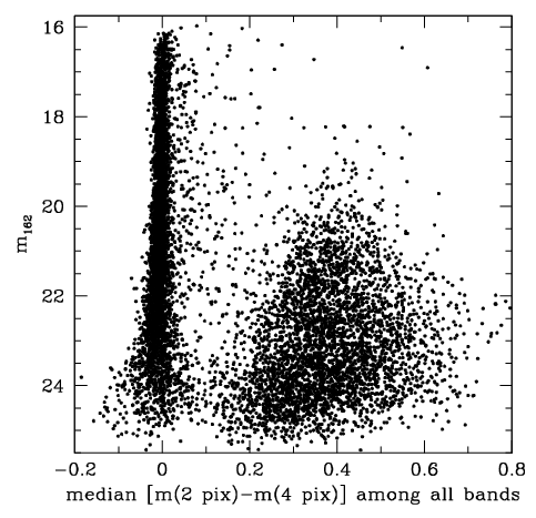
- How to read the axes and panels
- Magnitude is compared with an aperture-based morphology statistic. The dividing line is a catalogue-selection rule, not a physical transition in brown-dwarf atmospheres.
- What the plot is telling me
- A compact locus makes point-source selection practical, but its width and separation from extended objects should be read as a function of brightness. The faintest regime is exactly where a simple threshold may become less reliable.
- What it does not establish
- Being point-like is not cluster membership. An unresolved background object can pass the morphology test.
Source Figure 3 and original caption ↗ · CC BY 4.0; author/source attribution retained. No data, axes or annotations have been redrawn.
Colour selection and the results of follow-up
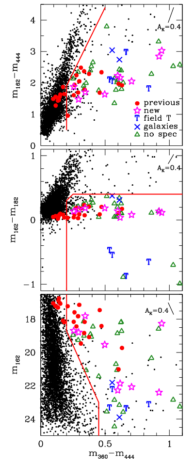
- How to read the axes and panels
- The colour–colour and colour–magnitude panels show selection boundaries, known members and candidates with later classifications.
- What the plot is telling me
- Track where confirmed members, background dwarfs and galaxies overlap. This reveals why a colour cut is a way to prioritise spectra rather than a final classification. The follow-up symbols let the reader evaluate the selection’s failure modes directly.
- What it does not establish
- Sources without spectra should not inherit the classifications of neighbouring points in the diagram. Proximity in a projected colour space does not establish a common physical nature.
Source Figure 4 and original caption ↗ · CC BY 4.0; author/source attribution retained. No data, axes or annotations have been redrawn.
An independent astrometric membership check
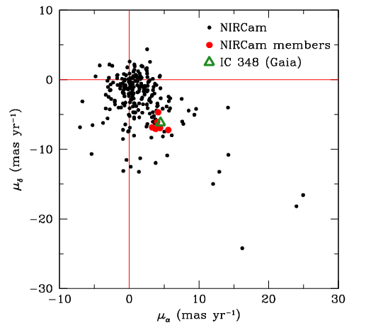
- How to read the axes and panels
- The axes are the two proper-motion components. Known members and a cluster reference can be compared with the wider field population.
- What the plot is telling me
- Clustering near an independently established motion supports membership for the objects actually measured. This is useful because it does not rely on the same spectral feature that motivates the new class.
- What it does not establish
- The two-epoch footprint does not include all newly selected candidates. This plot cannot be used as a membership measurement for sources absent from it.
Source Figure 6 and original caption ↗ · CC BY 4.0; author/source attribution retained. No data, axes or annotations have been redrawn.
The spectral evidence behind the proposed class
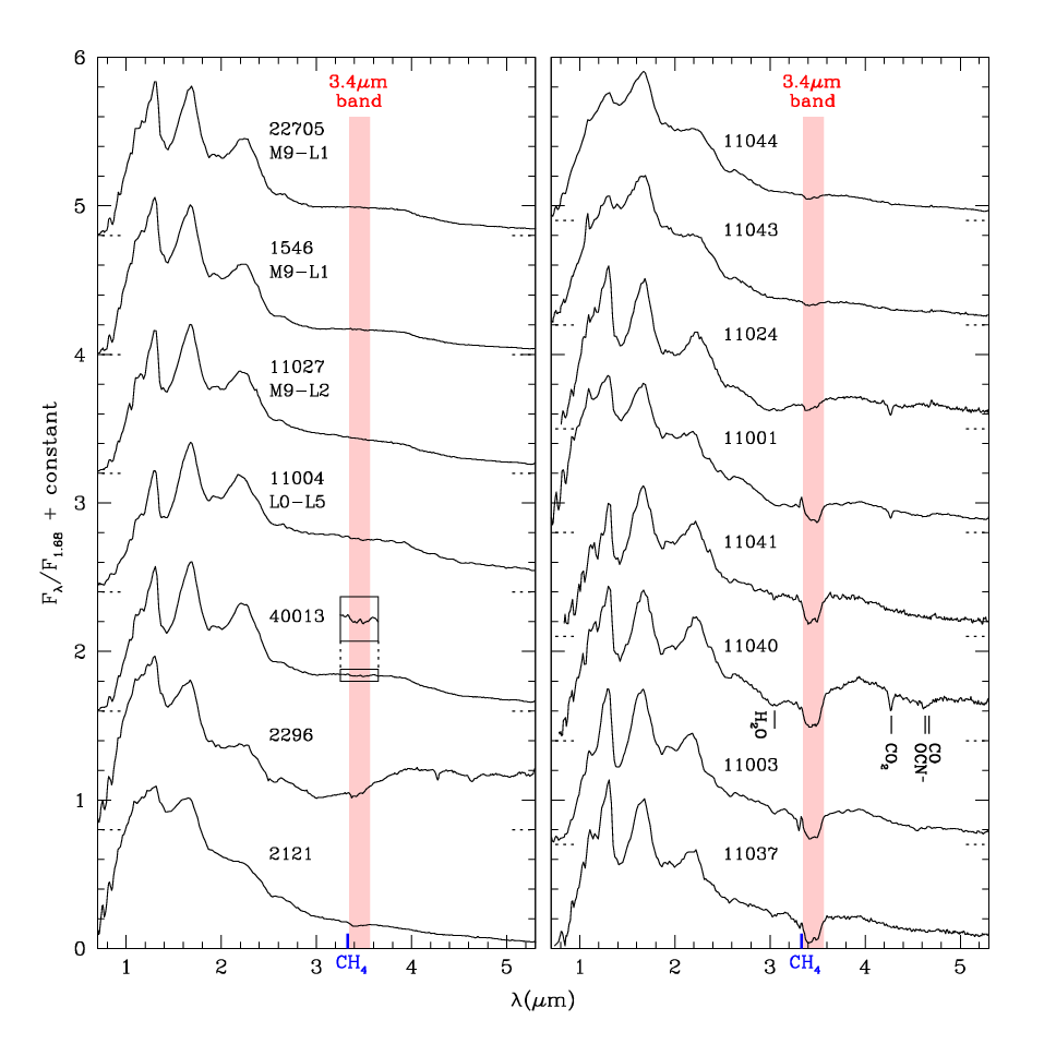
- How to read the axes and panels
- Wavelength runs horizontally, with spectra shifted for visibility and the hydrocarbon region highlighted. Zero-level marks and the methane reference help prevent misreading the offsets.
- What the plot is telling me
- Compare feature morphology across the sequence, not absolute flux from the vertical stacking. The juxtaposition with normal young L-dwarf spectra makes the new absorption behaviour visible. Long-wavelength excesses should be considered separately from the photospheric sequence.
- What it does not establish
- Vertical offsets are not luminosity differences. A marked methane wavelength is not a methane detection, and an unidentified band does not uniquely determine its chemical carrier.
Source Figure 7 and original caption ↗ · CC BY 4.0; author/source attribution retained. No data, axes or annotations have been redrawn.
Band strength versus photometric brightness
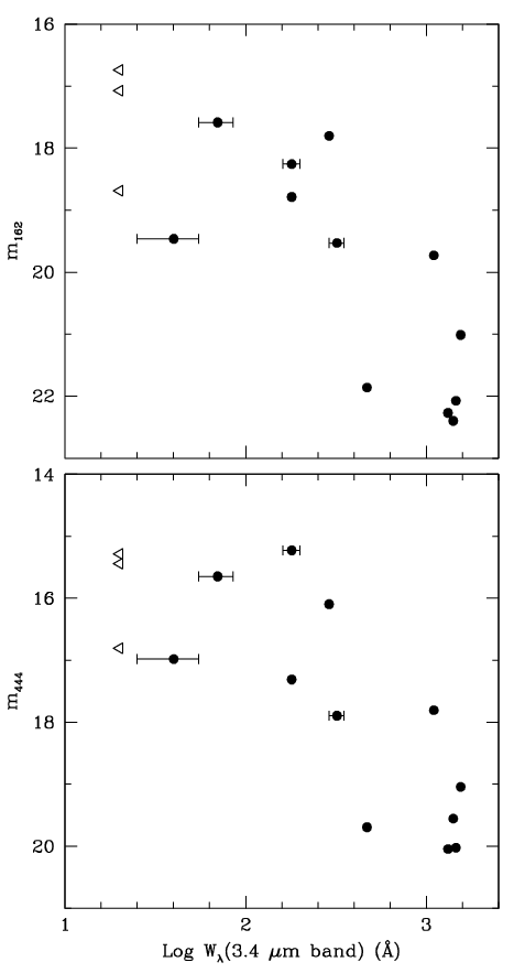
- How to read the axes and panels
- The panels compare the hydrocarbon equivalent width with photometry in two bands. Magnitude increases toward fainter sources, so the axis direction needs care.
- What the plot is telling me
- The relation supports the idea that the feature belongs systematically to this population rather than to a random foreground event. Read the uncertainty and the population trend, not just the most extreme object.
- What it does not establish
- Brightness is not a one-parameter temperature measurement. Extinction, disk emission and uncertain continua can affect an interpretation in terms of atmospheric abundance.
Source Figure 10 and original caption ↗ · CC BY 4.0; author/source attribution retained. No data, axes or annotations have been redrawn.
A luminosity-function view before converting to mass
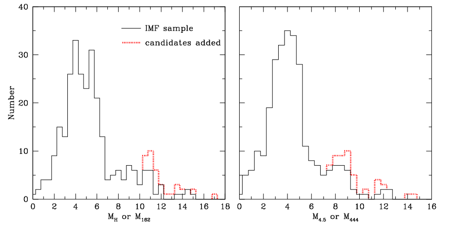
- How to read the axes and panels
- The histograms use extinction-corrected absolute magnitudes, with confirmed-sample and additional-candidate contributions distinguished.
- What the plot is telling me
- This is the more observational representation of the low-luminosity population. Comparing it with the mass-function figure exposes the role of the luminosity-to-mass conversion instead of hiding that modelling step.
- What it does not establish
- Absolute magnitude already assumes distance and extinction. Candidate additions and possible excess emission can alter bins without establishing a new population endpoint.
Source Figure 11 and original caption ↗ · CC BY 4.0; author/source attribution retained. No data, axes or annotations have been redrawn.
The inferred IMF and the role of unconfirmed candidates
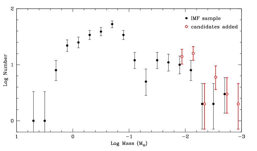
- How to read the axes and panels
- The mass-function points distinguish the adopted member sample from a version including remaining viable candidates. A small horizontal display shift is used for clarity.
- What the plot is telling me
- The separation of those two cases is scientifically useful: it shows how incomplete classification could change the low-mass tail. The interesting constraint is that the observed distribution reaches very low inferred masses, not that every added candidate is already confirmed.
- What it does not establish
- These are model-based mass estimates. The lowest observed point is not proof of a sharp physical fragmentation cutoff or a complete census below that mass.
Source Figure 12 and original caption ↗ · CC BY 4.0; author/source attribution retained. No data, axes or annotations have been redrawn.
Sources and scope
- Luhman & Alves de Oliveira (2025). A new spectral class of brown dwarfs at the bottom of the IMF in IC 348. Read the version used: arXiv:2506.08969v1 · Abstract and version history.
This is a selective literature-reading note. Source claims appear in “What the authors report”; the comparison table, conceptual chain and proposed tests are analytical commentary. No new observations, reanalysis or experimental validation are claimed. Expanded source review: 21 October 2026.