What the authors report
Chen et al. select 27 photometric candidates in the 0.243 deg² COSMOS-Web area studied: 25 T-type and two Y-type candidates. Selection uses NIRCam colours, morphology, visual checks and SED fitting. In AB magnitudes the cuts are F115W − F277W + 1 < F277W − F444W and F277W − F444W > 0.9. Sonora-Bobcat, ATMO2020++ and LOWZ fits yield model-dependent distances of roughly 0.3–4 kpc. The cumulative counts are consistent with the adopted double-exponential Galactic model. These remain candidates requiring spectroscopic follow-up, not 27 confirmed new brown dwarfs. [1]
Reading the evidence
| Stage | What it contributes | Possible sensitivity |
|---|---|---|
| Colour selection | A tractable candidate set. | Photometric scatter and model coverage. |
| Morphology | Rejection of resolved contaminants. | PSF variation and faint-source ambiguity. |
| Atmosphere fitting | Physical hypotheses and distance estimates. | Model family, degeneracies and radius assumptions. |
| Number-count comparison | A population consistency test. | Selection, contamination and accessible volume. |
The measurement chain
A conceptual reading aid, not measured data or a reproduction of a paper figure:
- Measured fluxes and errors
- Selection and contamination model
- Atmosphere-dependent distances
- Forward-modelled counts
Colour cuts must be propagated with their errors
A source close to a selection boundary can move in or out under plausible photometric perturbations. The same band appears in more than one colour, so the errors of those colours are correlated. Treating them as independent can misrepresent the selection probability.
I would perturb the underlying flux measurements, preserve any available covariance, and rerun the complete selection. Non-detections should enter through an appropriate likelihood or limit treatment rather than being converted into exact magnitudes.
A narrow posterior is not a model-independent distance
A schematic flux scaling is F_obs = (R/d)² F_surface. If radius is assumed rather than measured, the inferred distance inherits that assumption. Atmosphere parameters can also trade off against one another when only a few broad bands constrain the spectral shape.
More MCMC samples improve exploration of the chosen model; they do not remove a model degeneracy or make an incomplete atmosphere grid correct. I would compare posterior structure across model families and keep differences between families separate from within-model statistical uncertainty.
Number counts require a selection function
A useful forward model is N_exp = ∫ρ(r,Ω) S(r,θ,Ω) r² dr dΩ dθ, where S includes detection and selection probability and θ represents source properties. This makes explicit why a catalogue count alone is not a space density.
The survey’s ability to detect a source may vary across the footprint and with spectral shape. Contaminants alter the numerator; incompleteness alters the effective sampled population. Both should be carried into any comparison with Galactic structure, rather than hidden in one nominal volume.
How I would strengthen the inference
Recovery map: inject synthetic point sources across backgrounds and magnitudes, then rerun detection, photometry, morphology and colour selection together.
Contaminant comparison: evaluate brown-dwarf and galaxy hypotheses with a common likelihood and consistent upper-limit treatment. A lower best-fit χ² is not by itself a calibrated membership probability.
Model sensitivity: repeat the count comparison under plausible atmosphere, radius and Galactic-population choices. Inspect whether the scientific conclusion changes more than the formal counting error.
Targeted spectroscopy: prioritise candidates that distinguish competing models or occupy the uncertain tails of the inferred distance and temperature distributions, not simply the brightest objects.
Connection to the IC 348 note
The two papers probe different regimes. A cluster study benefits from shared distance and approximate age, whereas a deep field sample has a broader distance and population mixture. Their classifications and completeness boundaries should not be merged uncritically.
For a follow-up project, a transparent candidate table with alternate model fits, flags and recovery probabilities would be a useful first product. It would support later spectroscopy without presenting provisional photometric inference as settled discovery.
Following the full technical argument
The effective survey is defined by the bands actually available
The usable footprint is the region with the measurements needed by the selection, not simply the headline area of the parent survey. A missing band can remove a tile from a colour-selected search even if that tile still contains excellent images in other filters. This is an important connection between data engineering and population inference.
The method combines a detection-band catalogue with cross-band matches, colour cuts, morphological checks, ancillary imaging and template fitting. The order matters because each stage changes the surviving sample. A reproducible implementation should preserve the rejected population and a reason code, not only the final attractive candidates.
Morphological classifiers are brightness-dependent. A threshold that cleanly separates bright point sources from extended galaxies may be poorly calibrated at the faint limit. The use of multiple diagnostics helps, but does not turn a faint unresolved source into a confirmed brown dwarf. That still needs a physical classification argument and, ideally, spectroscopy.
SED fitting is a comparison between constrained hypotheses
Broad-band photometry measures integrals through filter responses rather than a resolved atmospheric spectrum. Different model spectra can therefore have nearly the same measured colours while differing strongly in an unobserved wavelength interval. This is why the paper’s model-family comparisons matter as much as the best-fit curve.
Distance enters through the model luminosity or a radius-dependent scale factor. A posterior interval conditioned on one atmosphere grid does not include every uncertainty in that grid, the radius or the population prior. The distinction between within-model precision and between-model disagreement should remain visible in any candidate table.
The classification exercise is also more weakly constrained than an observed spectral type. For many sources the template comparison over the available near-infrared range uses very little photometric information. The T/Y labels are useful candidate descriptors, not a substitute for an actual spectrum. Additional photometry is most valuable where competing models predict different fluxes, rather than where all of them already agree.
The number-count comparison is more cautious than a density headline
A cumulative count N(<m) includes the same bright objects in every subsequent faint bin. Its neighbouring points are consequently correlated. Visual proximity to a smooth population curve should not be read as a long series of independent confirmations. Small-number uncertainty and the magnitude-dependent selection remain important.
The spectral-type-based and temperature-based selections are different experiments because they inherit different model assumptions. Comparing them is useful, but apparent agreement of one does not remove systematic uncertainty in the other. The figure should be read with the selection definition attached to each panel.
Proper motion adds evidence for nearby Galactic sources where archival positions permit a measurement. A transverse velocity requires both angular motion and a distance estimate; it is not a radial velocity or a complete three-dimensional orbit. For future work I would combine recovery experiments, population modelling and spectroscopy before using the sample to infer a precise scale height or an unusual halo fraction.
Reading based on the full manuscript, including methods and discussion—not only its abstract. These explanations are original commentary; they are not a reproduced analysis or new experiment. Original manuscript · expanded 21 October 2026.
Paper plots, explained in detail
Read the paper plots alongside the explanations below. Each discussion keeps its source figure number and links to the original caption and context. Openly licensed panels are shown here; other figures open at the original paper. The explanations distinguish the plotted evidence from what it cannot establish.
Why the filters can identify a distinctive SED shape
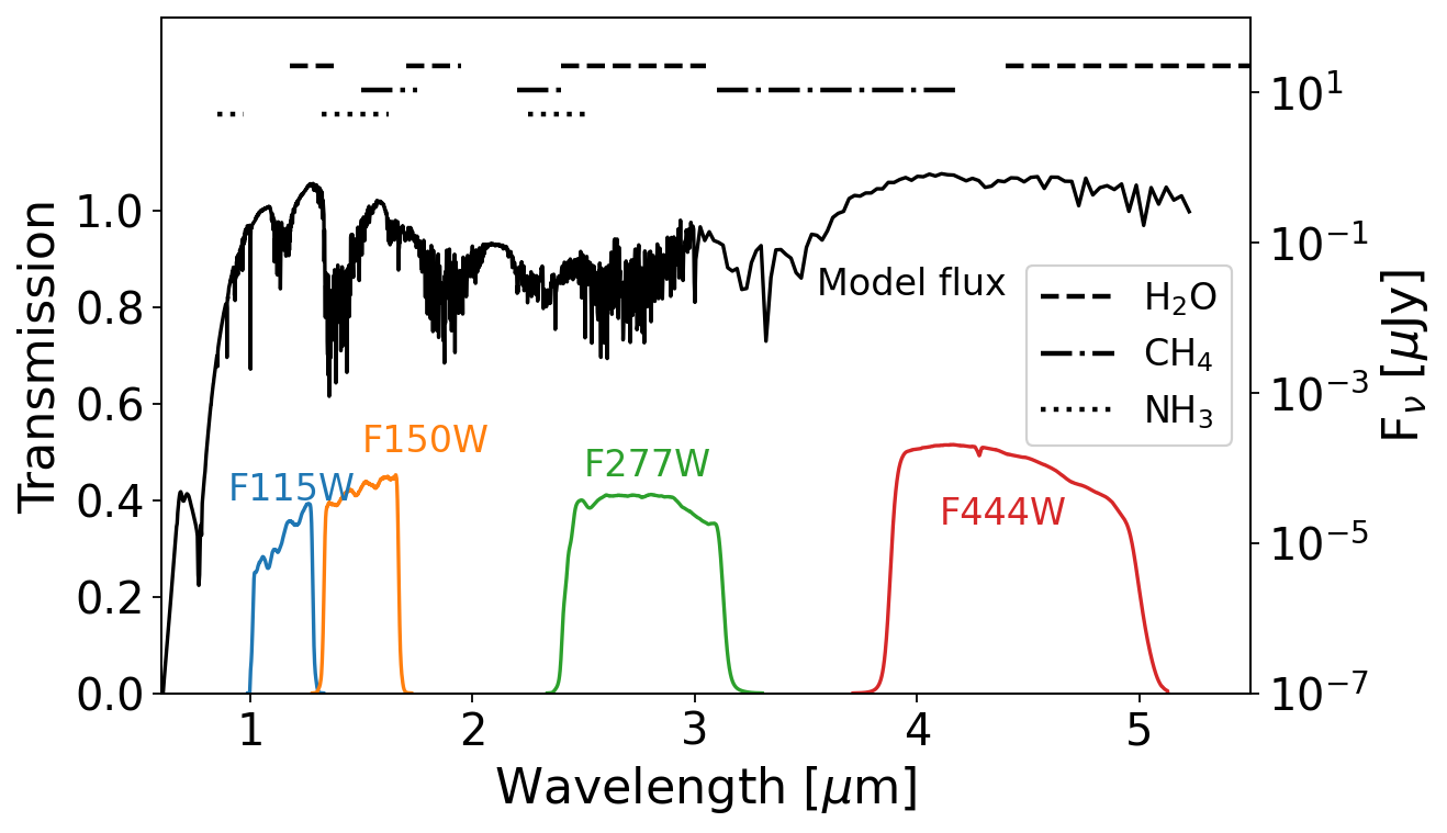
- How to read the axes and panels
- A model spectrum is plotted with NIRCam transmission bands and molecular-absorption regions. The filter curves describe wavelength weighting, not extra measured spectral points.
- What the plot is telling me
- The figure explains why a broad colour combination can respond to molecular structure. It also shows the information that is lost: a band averages over a finite wavelength range, so different detailed spectra may give similar photometry.
- What it does not establish
- The illustrated model is a fitted hypothesis, not a spectrum observed at every plotted wavelength. Do not count its fine structure as independent confirmation.
Source Figure 1 and original caption ↗ · CC BY 4.0; author/source attribution retained. No data, axes or annotations have been redrawn.
The colour boundary and atmosphere-model families
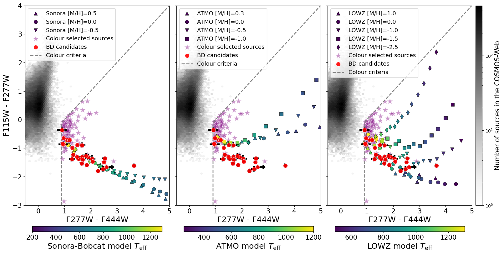
- How to read the axes and panels
- The panels compare observed colours with different model grids. Colour encodes model temperature, and the candidate error bars or limits describe observational uncertainty.
- What the plot is telling me
- Inspect where the models overlap and where candidates lie relative to the boundaries. The plot motivates a useful selection, while also exposing model dependence and the importance of non-detections. A point near a line should be treated probabilistically, not as an exact binary truth.
- What it does not establish
- The displayed grid fixes some parameters. Its two-dimensional projection is not the full range of all atmosphere models or contaminant populations.
Source Figure 2 and original caption ↗ · CC BY 4.0; author/source attribution retained. No data, axes or annotations have been redrawn.
CLASS_STAR loses power toward the faint limit
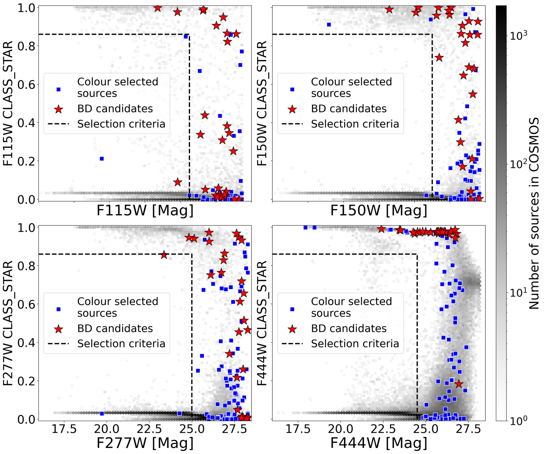
- How to read the axes and panels
- Each band compares the morphology classifier with magnitude. Candidate and preselection markers sit over the full source distribution.
- What the plot is telling me
- The important reading is where the point-like and extended populations remain distinguishable. A candidate’s high classifier value is stronger evidence in a well-separated bright regime than in a noisy faint one.
- What it does not establish
- This score is neither a brown-dwarf probability nor a spectroscopic classification. Calibration on one magnitude range should not be assumed to transfer unchanged to another.
Source Figure 3 and original caption ↗ · CC BY 4.0; author/source attribution retained. No data, axes or annotations have been redrawn.
A size-based cross-check
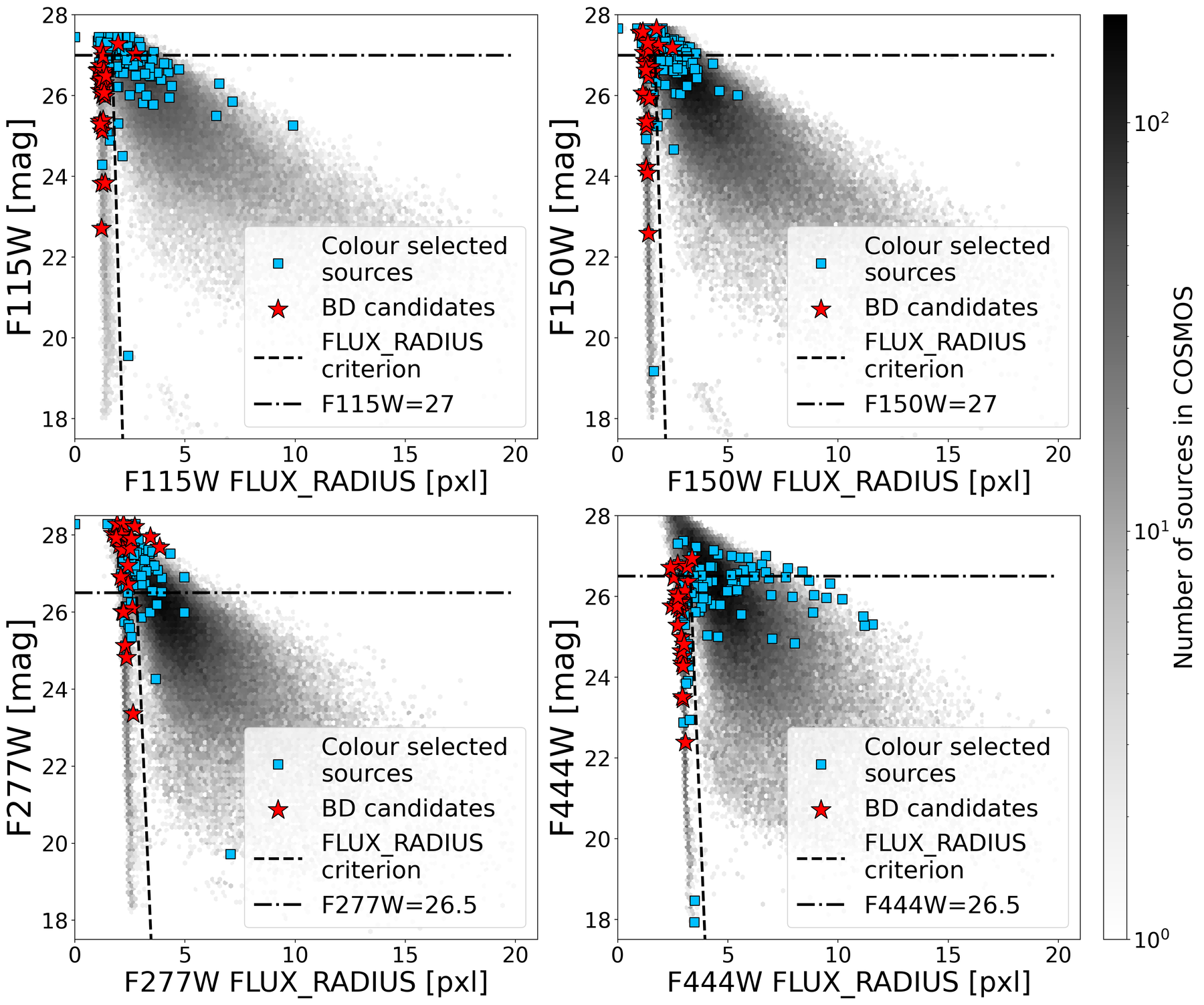
- How to read the axes and panels
- Flux radius is compared with magnitude in several filters, with thresholds marking the selection rule and its usable range.
- What the plot is telling me
- This supplies a second way to inspect whether a candidate is resolved. Read the local distribution and the magnitude limit together; the threshold is meaningful only where a size can be measured reliably.
- What it does not establish
- A point-source size does not distinguish a brown dwarf from every unresolved contaminant. PSF mismatch and faint-source noise can affect this diagnostic.
Source Figure 4 and original caption ↗ · CC BY 4.0; author/source attribution retained. No data, axes or annotations have been redrawn.
PSF-model consistency through SPREAD_MODEL
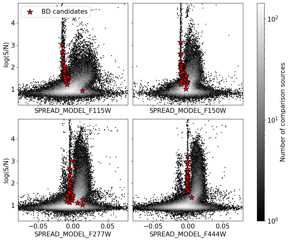
- How to read the axes and panels
- The panels relate a PSF-based morphology statistic to signal-to-noise, with the selected candidates shown against comparison sources.
- What the plot is telling me
- This figure checks whether the sample occupies the point-source-like population in another diagnostic space. It is most useful where that population is clearly separated, rather than as a decorative third confirmation of every candidate.
- What it does not establish
- A model PSF need not perfectly represent the mosaic. Small offsets in the point-source locus can be instrumental, and an unresolved galaxy or AGN can still require SED or spectral discrimination.
Source Figure 5 and original caption ↗ · CC BY 4.0; author/source attribution retained. No data, axes or annotations have been redrawn.
A representative candidate: fitted SED and image context
Selected BD01 panels only; the full multi-object figure is available at the source.
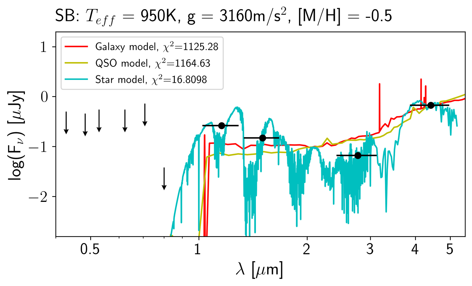
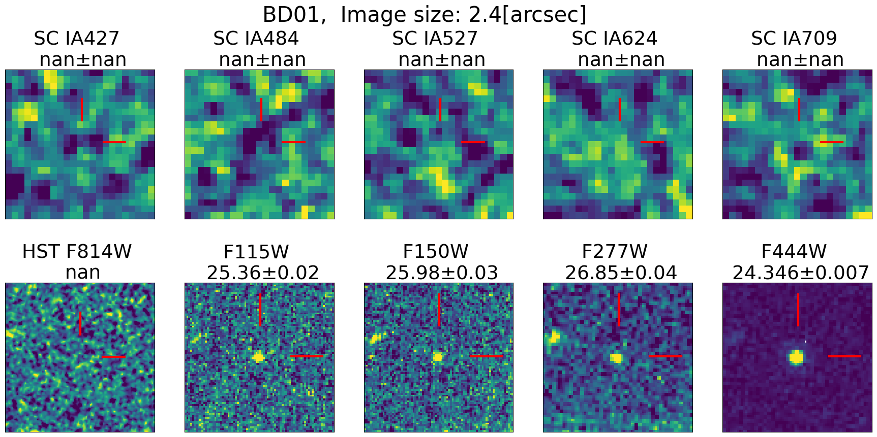
- How to read the axes and panels
- Only the BD01 SED panel and its associated cutout strip are shown here; this is an explicitly selected excerpt from a larger multi-object figure. Points, upper limits and alternative template curves have different evidential roles.
- What the plot is telling me
- Compare the templates at the measured bands and inspect the cutouts for blending or questionable detections. A visually convincing interpolated curve should not outweigh one problematic photometric point. The image context is an essential part of reading the fit.
- What it does not establish
- This representative example does not establish that every candidate has the same data quality. The full source figure and tables must be used for object-by-object conclusions.
Source Figure 6 and original caption ↗ · CC BY 4.0; author/source attribution retained. No data, axes or annotations have been redrawn.
Cumulative counts against a Galactic model
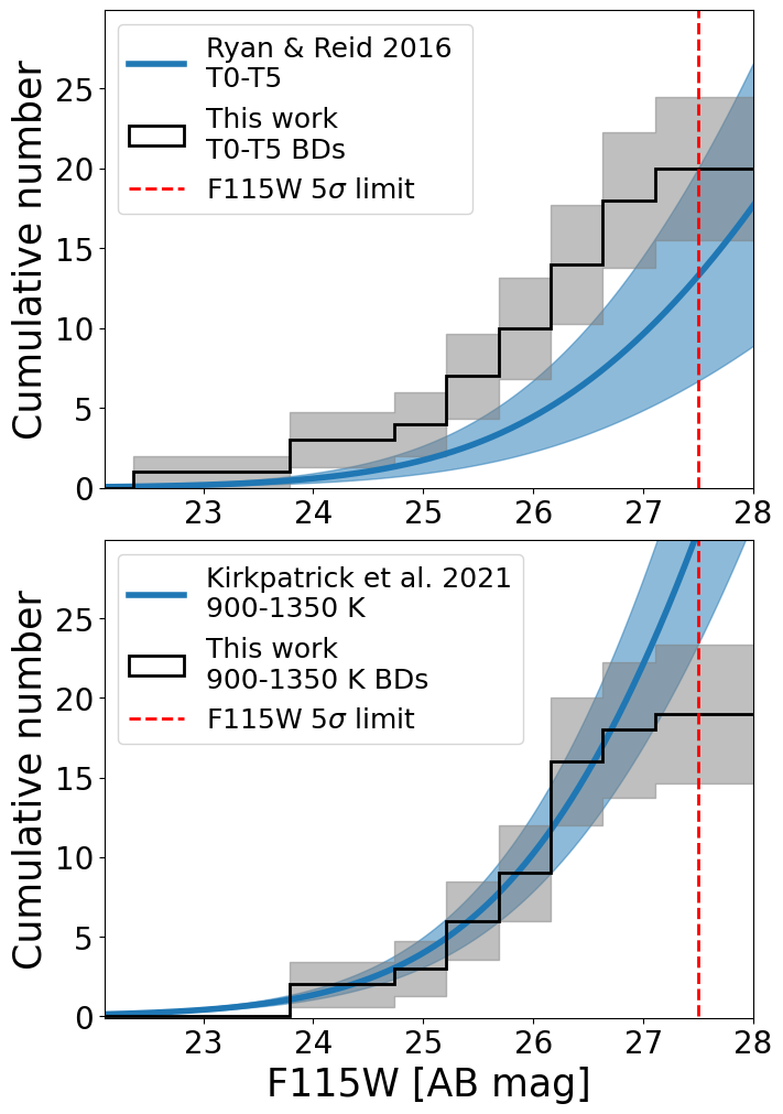
- How to read the axes and panels
- The upper and lower panels use different population selections. Histograms, uncertainty bands, model predictions and a limiting-magnitude marker should be read together.
- What the plot is telling me
- Compare the observed progression toward fainter magnitudes with the predicted count curve, but remember that cumulative bins share objects. Agreement is a consistency check under the adopted sample and model, not a direct proof of the Galaxy’s density law.
- What it does not establish
- The sample is small and remains photometrically selected. Contamination, incomplete recovery and atmosphere-dependent classification can shift the comparison beyond the displayed counting uncertainty.
Source Figure 8 and original caption ↗ · CC BY 4.0; author/source attribution retained. No data, axes or annotations have been redrawn.
Sources and scope
- Chen et al. (2025). Brown dwarf number density in the JWST COSMOS-Web field. Read the version used: arXiv:2503.18510v2 · Abstract and version history.
This is a selective literature-reading note. Source claims appear in “What the authors report”; the comparison table, conceptual chain and proposed tests are analytical commentary. No new observations, reanalysis or experimental validation are claimed. Expanded source review: 21 October 2026.