What is PID Control?

PID is the controller everyone uses because it is simple enough to implement, powerful enough to be useful, and annoying enough to tune properly.

Welcome to PID control: three letters, one feedback loop, and a surprising number of ways to make a system oscillate like it has unresolved emotional issues.

2026-05-08 · Hertford, London, UK 12 min read Interactive PID response lab

PID turns error into correction using the present, the past, and the trend.

A PID controller calculates a control action from three ingredients: proportional response to current error, integral response to accumulated error, and derivative response to the rate of change. It is not magic. It is a practical compromise that became everywhere because it works surprisingly often.

Chapter 01 · P

Proportional control reacts to what is wrong right now.

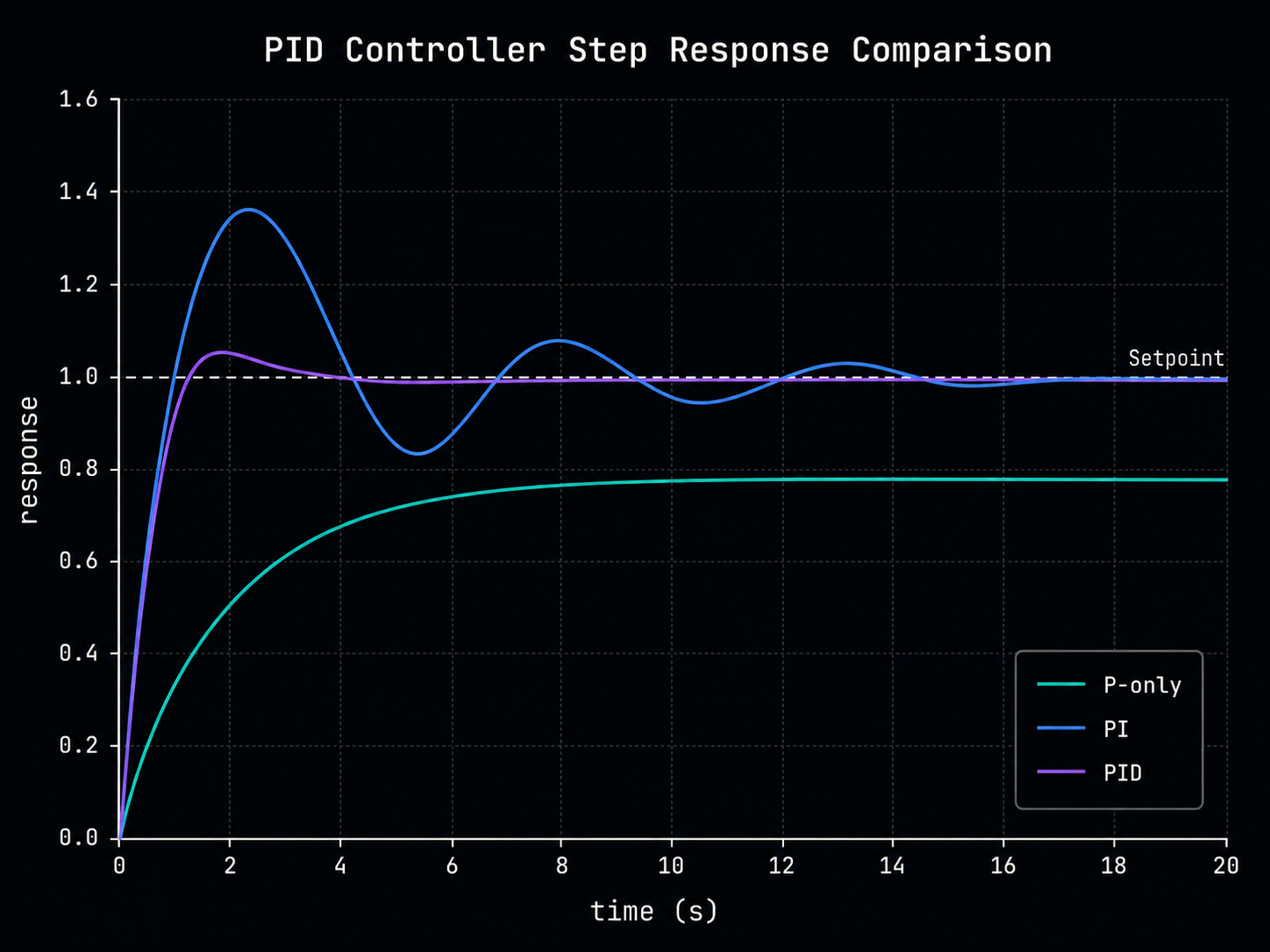
The proportional term scales with the present error. If the output is far from the setpoint, the correction is large. If the output is close, the correction is small. This is intuitive and often effective, but P-only control usually leaves a steady-state offset.

Proportional term

\[u_P(t)=K_p e(t)\]

Large \(K_p\) gives stronger response but can also create overshoot and oscillation.

Chapter 02 · I

The integral term remembers old mistakes.

The integral term accumulates error over time. If a small offset persists, the integral grows until the controller pushes the system closer to the setpoint. This eliminates steady-state error, but too much integral action can cause slow oscillation and windup.

Integral term

\[u_I(t)=K_i\int e(t)\,dt\]

The integral term is powerful because it refuses to forget persistent error. Unfortunately, it sometimes refuses to forget too much.

Chapter 03 · D

The derivative term tries to brake before the crash.

The derivative term responds to how quickly the error is changing. It can reduce overshoot by damping the response. But because differentiation amplifies high-frequency noise, derivative control must be used carefully.

Derivative term

\[u_D(t)=K_d\frac{de(t)}{dt}\]

Derivative action is useful when the measurement is clean enough not to turn every tiny noise spike into a dramatic correction.

Chapter 04 · Tuning

Tuning is where polite equations meet rude hardware.

The full PID controller combines all three terms. Increasing gains can improve response, but also risks overshoot, oscillation, actuator saturation, and instability. Good tuning balances speed, damping, and robustness.

PID control law

\[u(t)=K_p e(t)+K_i\int e(t)\,dt+K_d\frac{de(t)}{dt}\]

The output \(u(t)\) is the sum of present, accumulated, and predictive corrections.

A PID controller is easy to write. A good PID controller is the part where humility enters the laboratory.

Chapter 05 · Implementation

Real PID is discrete, noisy, and bounded.

In real systems the controller runs at discrete time steps. Sensors are noisy. Actuators saturate. Delays exist. Anti-windup, filtering, output clamps, and safe limits matter as much as the ideal equation.

Discrete approximation

\[u[n]=K_p e[n]+K_iT_s\sum e[k]+\frac{K_d}{T_s}(e[n]-e[n-1])\]

\(T_s\) is the sampling interval. In software, this is the version that actually gets to meet reality.

Takeaway

PID is simple because it has to be.

Its strength is not theoretical perfection. Its strength is practical clarity: respond to the error, remember persistent bias, and damp fast change. That is why PID remains one of the most useful algorithms in engineering.