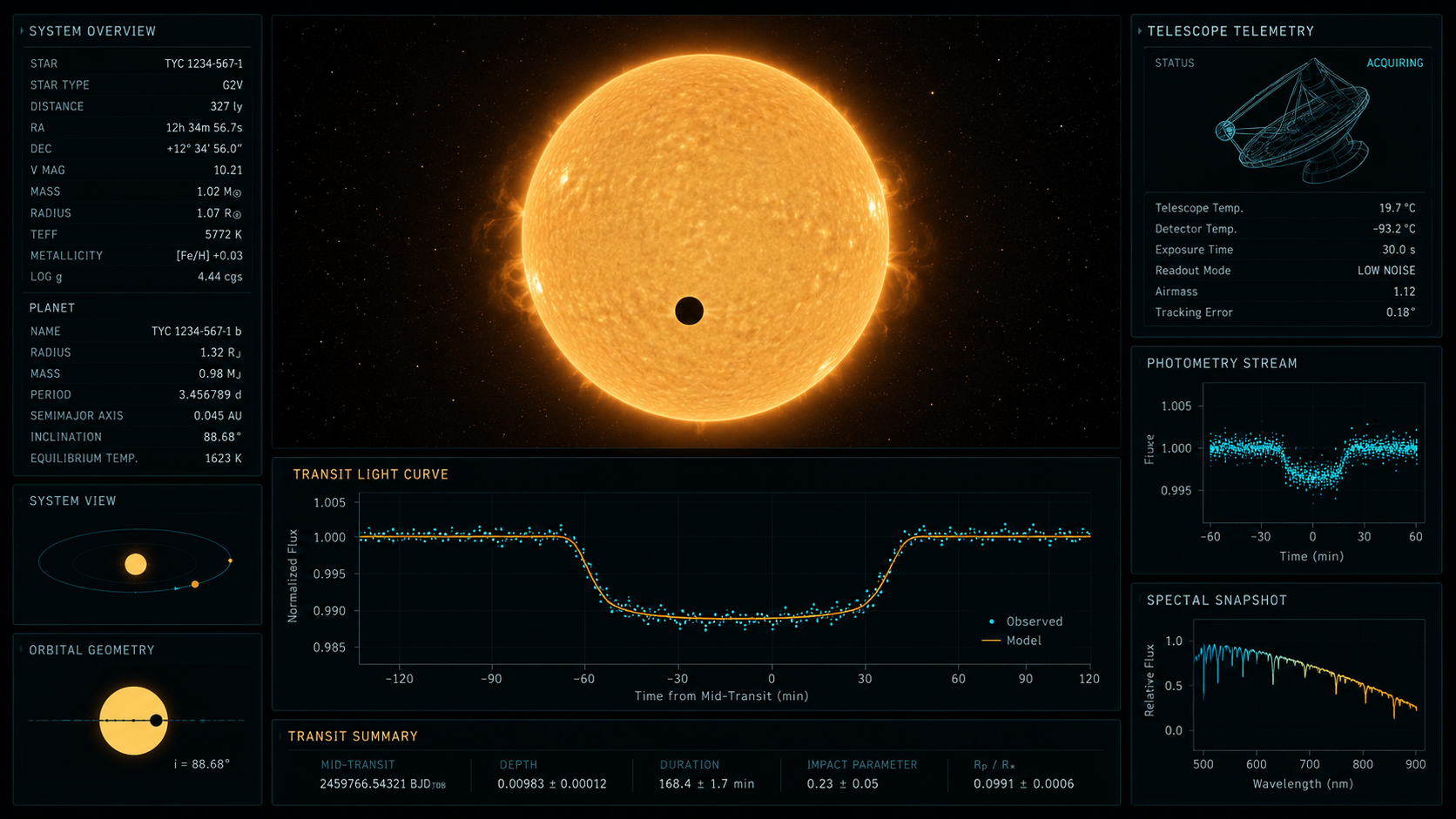
Transit photometry now dominates the confirmed exoplanet census.
The scale of the field is now enormous. As of the NASA Exoplanet Archive update used for this article, the archive listed 6,287 confirmed exoplanets. Of these, 4,648 were attributed to the transit discovery method, and 4,690 were listed as transiting exoplanets. That means the transit method is not a niche technique; it is the main engine behind the modern planet census.
The candidate numbers are just as important. A candidate is not a confirmed planet; it is a signal that looks planet-like enough to deserve further vetting. The archive listed 1,978 Kepler project candidates still awaiting confirmation, 976 K2 candidates still awaiting confirmation, and 7,931 TESS project candidates integrated into the archive. TESS candidates that had not yet been dispositioned as confirmed planets or false positives numbered 4,783.
| Survey / category | Count | Interpretation |
|---|---|---|
| Kepler confirmed planets | 2,784 | Planets discovered using Kepler observations and published/validated as confirmed. |
| Kepler candidates yet to confirm | 1,978 | KOI signals still awaiting confirmation or rejection. |
| K2 confirmed planets | 549 | Confirmed planets from the extended Kepler/K2 mission. |
| K2 candidates yet to confirm | 976 | Candidate signals from K2 still needing disposition. |
| TESS confirmed planets | 893 | TESS planets published in refereed literature and counted by the archive. |
| TESS project candidates | 7,931 | Transit-like events identified by the TESS project, including false positives. |
| TESS candidates yet to confirm | 4,783 | TESS project candidates not yet confirmed or labelled as false positives. |
What is the transit method?
The transit method detects planets by measuring tiny, periodic decreases in a star's brightness. The star is not physically turning off. A planet is temporarily blocking a fraction of the visible stellar disk. To a telescope, the planet appears as a moving mask across a luminous surface.
The signal is usually shallow. A Jupiter-sized planet crossing a Sun-sized star blocks about one percent of the light. An Earth-sized planet crossing a Sun-sized star blocks only about 84 parts per million. That is why space telescopes, careful detrending, and repeated events matter.
If the stellar disk were uniformly bright and the planet were fully in front of it, the fractional loss of light would be roughly the area ratio between the planet and the star.
The geometry has to be lucky.
A planet can orbit a star without ever transiting from our point of view. A transit requires the orbital plane to line up with our line of sight so the planet crosses the stellar disk. The closer the orbit is to edge-on, the more likely we are to see a transit.
The impact parameter describes how far the transit chord passes from the stellar centre. A central transit crosses the bright central region and usually has a longer, deeper, more symmetric shape. A grazing transit skims the limb and can be shallow, V-shaped, and harder to distinguish from an eclipsing binary.
Here \(a\) is the orbital semi-major axis, \(i\) is inclination, and \(R_\star\) is stellar radius. For eccentric orbits, \(e\) and \(\omega\) also enter the geometry.
The light curve is the fingerprint.
A clean transit has four contact points: first contact when the planet touches the stellar limb, second contact when the full planet disk is inside the stellar disk, third contact when egress begins, and fourth contact when the planet leaves. The time between first and fourth contact is the total transit duration.
The light curve is not a perfect box. Stars are limb-darkened: their apparent disks are brighter at the centre and fainter near the edge. This changes the slope of ingress and egress and can shift the relationship between depth and \(R_p/R_\star\).
In detailed modelling, limb-darkening coefficients depend on stellar effective temperature, surface gravity, metallicity, and observing bandpass.
What can we learn from a transit?
The most direct measurement is the planet's size relative to the star. If the stellar radius is known, the transit depth gives an estimate of the planet radius. The repeated timing gives the orbital period. Combining the period with stellar mass gives the orbital scale through Kepler's third law.
A transit alone normally does not give mass. For that, we usually need radial velocity measurements, transit timing variations in multi-planet systems, or other dynamical constraints. Once mass and radius are both known, the bulk density tells us whether a planet is likely rocky, gaseous, icy, or intermediate.
Since \(M_p\ll M_\star\) for most planets, the stellar mass dominates the orbital solution.
Real light curves are not polite.
A textbook transit is clean. Real data rarely are. Stars rotate, pulsate, flare, and carry spots across their surfaces. Instruments drift. Detectors have systematics. Spacecraft momentum dumps, scattered light, cosmic rays, and background stars can all complicate the signal.
A candidate becomes convincing when the signal repeats with a consistent period, duration, and depth, and when the false-positive tests do not reveal a better explanation. Astronomers check odd-even transit depths, secondary eclipses, centroid motion, nearby contaminating stars, colour dependence, high-resolution imaging, and spectroscopic follow-up.
From detection to atmospheric physics.
During a transit, a small fraction of starlight passes through the planet's atmosphere before reaching us. Atoms and molecules absorb specific wavelengths, so the apparent transit depth can change with wavelength. This is transmission spectroscopy.
The signal is tiny, but it can reveal atmospheric species, clouds, hazes, atmospheric escape, and temperature structure. Transit detections therefore do more than find planets: they identify targets for JWST and future observatories to study as physical worlds.
Atmospheric absorption can make the planet appear slightly larger at wavelengths where the atmosphere is more opaque.
The method is powerful, but not universal.
Transit surveys are biased toward planets that are large, close to their stars, and frequently transiting. Small long-period planets are harder because they produce shallower dips and require long observing baselines to detect multiple events.
The method also depends on alignment. Most planetary systems are not oriented so that every planet transits from Earth. This does not make the method weak; it means transit detections are geometrically selected samples that must be interpreted carefully.
Why I built a transit lab.
Static figures explain the idea, but they hide the sensitivity of the method. Change \(R_p/R_\star\), and the depth changes. Increase the impact parameter, and the shape changes. Add limb darkening, and the curve becomes less box-like. Add a moon-like body or a starspot, and the residuals start telling a more complicated story.
That is the motivation behind ExoIntel-Prime: to make the geometry visible, the light curve responsive, and the physics less abstract. It is not a replacement for professional fitting pipelines, but it is a bridge between textbook formulas and live scientific modelling.
References and data sources
- NASA Exoplanet Archive. Exoplanet and Candidate Statistics. Archive statistics page.
- NASA Exoplanet Archive. Homepage count summary. NASA Exoplanet Archive.
- Seager, S. and Mallén-Ornelas, G. (2003). A unique solution of planet and star parameters from an extrasolar planet transit light curve.
- Mandel, K. and Agol, E. (2002). Analytic light curves for planetary transit searches.
- Charbonneau, D. et al. (2000). Detection of planetary transits across a Sun-like star.
- Brown, T. M. et al. (2001). Hubble Space Telescope time-series photometry of the transiting planet of HD 209458.
- Borucki, W. J. et al. (2010). Kepler Planet-Detection Mission: Introduction and first results.
- Ricker, G. R. et al. (2015). Transiting Exoplanet Survey Satellite.
- Winn, J. N. (2010). Exoplanet transits and occultations.
Comments and reactions
Comments are powered by GitHub Discussions through giscus. You can leave a question, correction, or reaction below.