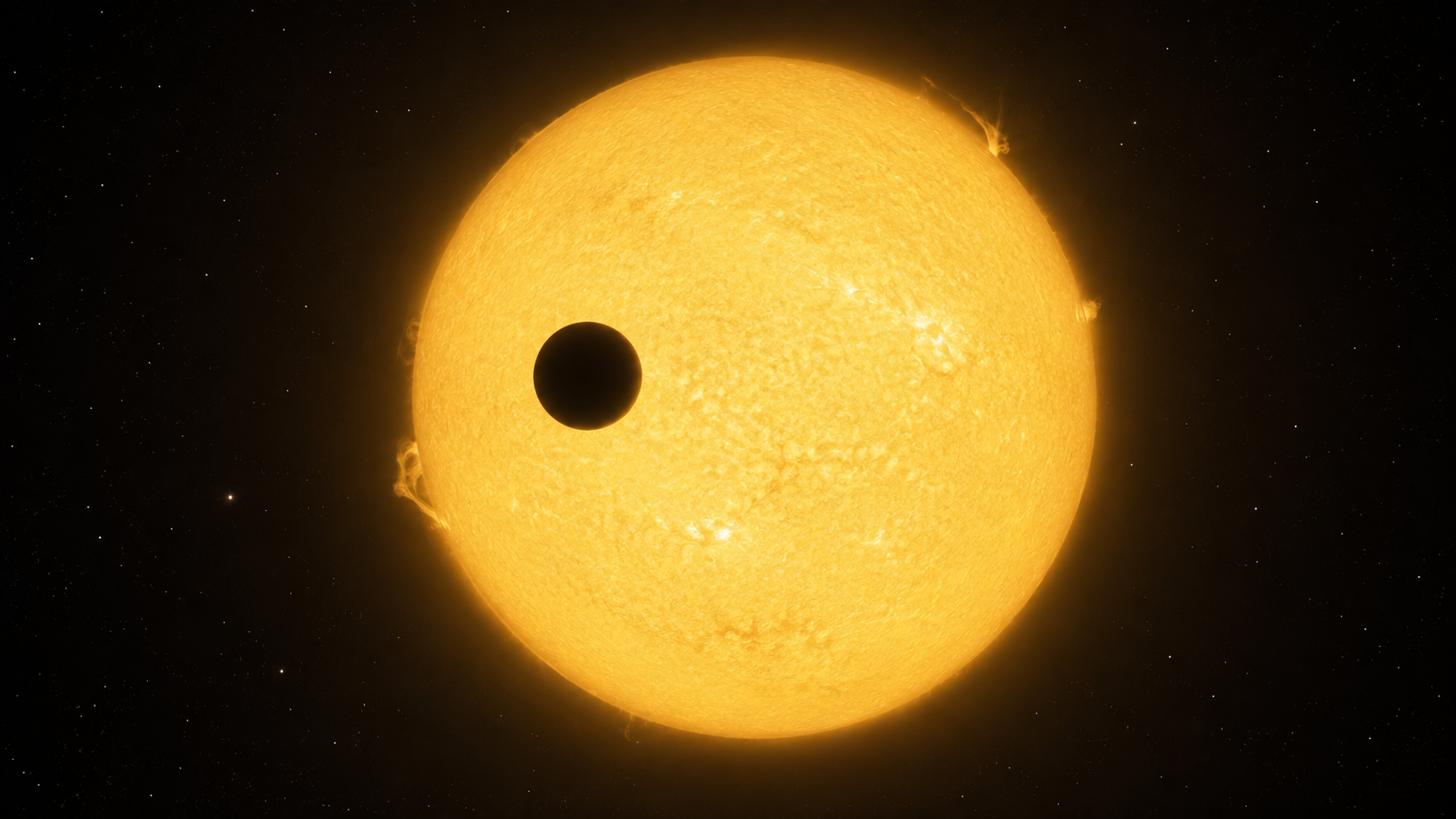
AI-generated artist's concept — not a real photograph. See the report for actual Kepler/TESS data.
How the majority of known exoplanets have been found: watching a star's brightness for the tiny, periodic dip caused by a planet passing in front of it. This repo works through the physics and statistics of the method and implements a Box Least Squares (BLS) period search — a standard, widely used transit-search algorithm, related in purpose to but not the same as the adaptive wavelet matched-filter architecture the actual Kepler and TESS mission pipelines use — from scratch in Python, searching period, phase, *and* duration blind, then validated by injecting a known signal and recovering it. **[Open the full report](https://biswajit1999.github.io/transit-photometry-detection-method/)** — the live GitHub Pages version. You can also open `index.html` locally in a browser, or serve it with `python -m http.server` from this directory. Related, from the same author: [ExoIntel-Prime / exolight-transit-lab](https://biswajit1999.github.io/exolight-transit-lab/), an earlier transit-photometry lab covering related light-curve analysis. ## The physics ### Why the star gets dimmer, and by how much When a planet of radius $R_p$ transits a star of radius $R_\star$, it blocks a fraction of the starlight equal to the ratio of their disk areas — the planet's silhouette against the star's: $$\delta \approx \left(\frac{R_p}{R_\star}\right)^2$$ For an Earth-Sun-like pair this is about 84 parts per million; for a Jupiter-Sun-like pair it's roughly 1%. That's the entire signal a transit survey is trying to detect: a fractional dimming often smaller than the star's own natural brightness fluctuations, which is why transit searches need long, uninterrupted, high-cadence monitoring. ### How long a transit lasts The transit duration depends on the orbital period $P$, the star's radius, the orbital semi-major axis $a$, and the impact parameter $b$ (how centrally the planet crosses the star's disk, in units of stellar radii — $b=0$ is a straight line through the center, $b$ near 1 is a grazing transit): $$T_{dur} \approx \frac{P}{\pi} \arcsin\left(\frac{R_\star}{a}\sqrt{(1+R_p/R_\star)^2 - b^2}\right)$$ For a close-in planet this is typically hours; the ratio of transit duration to orbital period is small, which is part of why a period search has to check many candidate periods and phases before it finds one where a box actually lines up with real dips. ### Ingress, egress, and limb darkening A real transit isn't a perfect box: the star dims gradually as the planet's disk moves onto the star (ingress) and brightens gradually as it moves off (egress), and the star itself is dimmer at its limb than its center (limb darkening), which smooths and slightly reshapes the dip further. Detailed transit-shape fitting (e.g. the Mandel & Agol 2002 analytic model) accounts for this; a box-shaped search like BLS is a deliberately simpler first-pass detection tool that trades shape accuracy for search speed, then hands promising candidates off to a full transit-shape fit. ### Why three transits, not one A single dip in a light curve can come from an instrumental artifact, a starspot rotating across the disk, or a background eclipsing binary blended into the same pixel — not just a planet. Requiring at least three transits at a consistent period, depth, and duration is the standard first bar for calling a signal a genuine planet candidate, since coincidentally reproducing all three by chance gets increasingly unlikely with each repeat. ## Why this method dominates the exoplanet census Transit photometry needs only a stable, well-calibrated brightness measurement — no need to resolve the star and planet separately, and no need for the extreme spectral precision radial velocity requires. This makes it well suited to wide-field surveys that monitor huge numbers of stars simultaneously. Per the NASA Exoplanet Archive's confirmed-planet counts by discovery method (accessed 2026-08-14), transit photometry accounts for 4,676 of 6,336 confirmed exoplanets (~74%) — by a wide margin the most productive method in the field's history, driven almost entirely by three purpose-built space missions: | Method | Confirmed count | Share | |---|---|---| | Transit | 4,676 | ~74% | | Radial velocity | 1,197 | ~19% | | Microlensing | 282 | ~4% | | Direct imaging | 98 | ~2% | | All other methods (TTV, ETV, pulsar/pulsation timing, astrometry, disk kinematics) | 83 | <2% | Primarily via **Kepler** (2009-2018, continuous staring survey of one ~115 deg² field), **K2** (Kepler's repurposed extended mission, 2014-2018), and **TESS** (2018-present, all-sky survey). **Limitation:** transit photometry only detects planets whose orbits happen to be aligned edge-on as seen from Earth — a geometric probability of roughly $R_\star/a$, meaning it systematically undercounts real planetary systems whose orbits aren't so aligned, and it directly measures $R_p$, not mass (radial velocity or transit-timing follow-up is needed for that). ## What this repo's code does `scripts/transit_photometry_demo.py`: 1. Injects a known transit signal (period, depth, duration) into a synthetic light curve with Kepler's own published ~100 ppm per-30- minute photometric noise level for a quiet Sun-like star. 2. Implements Box Least Squares (Kovacs, Zsom & Mazeh 2002) from scratch: a search over trial period, trial phase offset, *and* trial duration (a grid of fractional durations, not the injected value), sliding a box across the folded light curve at each combination and keeping the one with the strongest signal residue — the same core logic used by the Kepler and TESS transit-search pipelines. 3. Recovers the period, phase, duration, and depth, and reports the error against the known injected values, plus an in-transit depth signal-to-noise ratio. Run it yourself: ```bash pip install -r requirements.txt python scripts/transit_photometry_demo.py ``` ## Tests `tests/test_transit_photometry.py` checks the transit model and BLS search directly — not just the one illustrative injection-recovery run above — including period recovery across multiple noise seeds. Runs automatically on every push via GitHub Actions; run locally with: ```bash pytest tests/ -v ``` ## Sanity check against a real target's published parameters The depth equation at the top of this README isn't just for the synthetic signal above — it applies directly to any real transiting planet. Take HD 209458 b, covered elsewhere in this portfolio (`hd209458b-exoplanet-report`): the NASA Exoplanet Archive gives its radius as 15.58 Earth radii and its host star's radius as 1.19 Solar radii. Plugging straight into $\delta \approx (R_p/R_\star)^2$: ``` Rp = 15.58 * 6371 km = 99,260 km Rstar = 1.19 * 695,700 km = 827,883 km depth = (99,260 / 827,883)^2 = 0.014375 = 14,375 ppm ``` The real JWST MIRI spectrum analyzed in that companion repo gives a weighted-mean measured depth of 14,458 ppm — a 0.6% difference from this two-line calculation. That's scale agreement between a bare geometric formula and a real measured spectrum, not a validation of the BLS search above (BLS was never run on this target here — this is a separate, static arithmetic check). The real spectrum's own wavelength dependence, plus limb darkening, impact parameter, and reduction-pipeline choices (see that repo's own analysis) account for the remaining difference. ## Result | Quantity | Injected | Recovered | Error | |---|---|---|---| | Period | 4.35 days | 4.3500 days | 0.00% | | Duration | 2.8 hours | 3.13 hours | 11.86% (searched blind over 6 fractions) | | Depth | 850.0 ppm | 833.8 ppm | 1.90% | | In-transit depth SNR | — | 77.8σ | uncorrected for search trials | The BLS period search cleanly isolates the true period against aliasing at harmonics/sub-harmonics (visible as smaller peaks in `figures/transit_bls_recovery.png`), and — without ever being told the true duration — recovers one close enough to produce a clean, box-shaped phase-folded transit. ## Limitations The quoted SNR is the in-transit depth signal-to-noise under the known Gaussian noise model at the recovered period/phase/duration; it is not a trial-corrected false-alarm probability accounting for the number of period/phase/duration combinations searched, which is what a real survey pipeline's significance threshold has to account for (the NASA Exoplanet Archive's periodogram service, for instance, defines an explicit minimum/maximum transit-duration-fraction search range and reports a separate false-alarm statistic). The synthetic light curve also has none of the red noise, data gaps, stellar variability, or systematics a real Kepler or TESS light curve carries, so recovery here is easier than a real low-SNR candidate search. ## Extending this To close some of that gap: add correlated ("red") noise to the synthetic light curve instead of pure Gaussian noise, introduce data gaps (real satellites have downlink and safe-mode interruptions), swap the box-shaped transit model for the Mandel & Agol (2002) limb-darkened analytic model, and run the whole pipeline hundreds of times on noise-only light curves (no injected transit) to build an empirical false-alarm-probability distribution for a given signal residue threshold — which is what turns a signal residue into an actual detection significance. Real implementations of this full pipeline exist in the `astropy.timeseries.BoxLeastSquares` module and the `transitleastsquares` package, both worth comparing your own BLS output against. ## Why this repo uses simulated (not raw archival) data This repo demonstrates the *method itself* — its sensitivity, biases, and failure modes — which is best shown with a known "ground truth" to validate recovery against. This portfolio's companion `*-exoplanet- report` repositories instead each analyze one real target's archival JWST/HST/Spitzer/ground-based spectra directly, with no simulated data. Both approaches are stated plainly here rather than blurring the two. ## Repository structure ```text scripts/transit_photometry_demo.py BLS implementation + injection-recovery test figures/ generated plot + summary_statistics.csv ``` ## References 1. Charbonneau, D. et al., 2000. Detection of Planetary Transits Across a Sun-like Star. *The Astrophysical Journal Letters*, 529(1), L45 — the first exoplanet transit detection (HD 209458 b). 2. Kovacs, G., Zsom, A. and Mazeh, T., 2002. A box-fitting algorithm in the search for periodic transits. *Astronomy & Astrophysics*, 391, pp.369-377. 3. Mandel, K. and Agol, E., 2002. Analytic Light Curves for Planetary Transit Searches. *The Astrophysical Journal Letters*, 580(2), L171. 4. Borucki, W.J. et al., 2010. Kepler Planet-Detection Mission: Introduction and First Results. *Science*, 327(5968), pp.977-980. 5. Ricker, G.R. et al., 2015. Transiting Exoplanet Survey Satellite (TESS). *Journal of Astronomical Telescopes, Instruments, and Systems*, 1(1), 014003. 6. NASA Exoplanet Archive periodogram service documentation,