Type Ia supernovae · distance · expansion history

A stellar explosion becomes a ruler for the Universe.

A Type Ia supernova can briefly rival the light of its host galaxy. Correct its light-curve width and colour, compare apparent with standardized luminosity, and it yields a distance. Repeat that measurement across redshift and the changing expansion rate appears in the Hubble diagram.

≈ −19.3 mag
typical standardized Type Ia peak absolute magnitude
≈ 10,000 km s⁻¹
characteristic photospheric ejecta velocity near maximum light
≈ 0.10–0.15 mag
standardized distance-modulus scatter in modern samples
1,701 / 1,550
Pantheon+ light curves / distinct supernovae

What is a supernova?

A rapid stellar disruption; a long-lived expanding remnant.

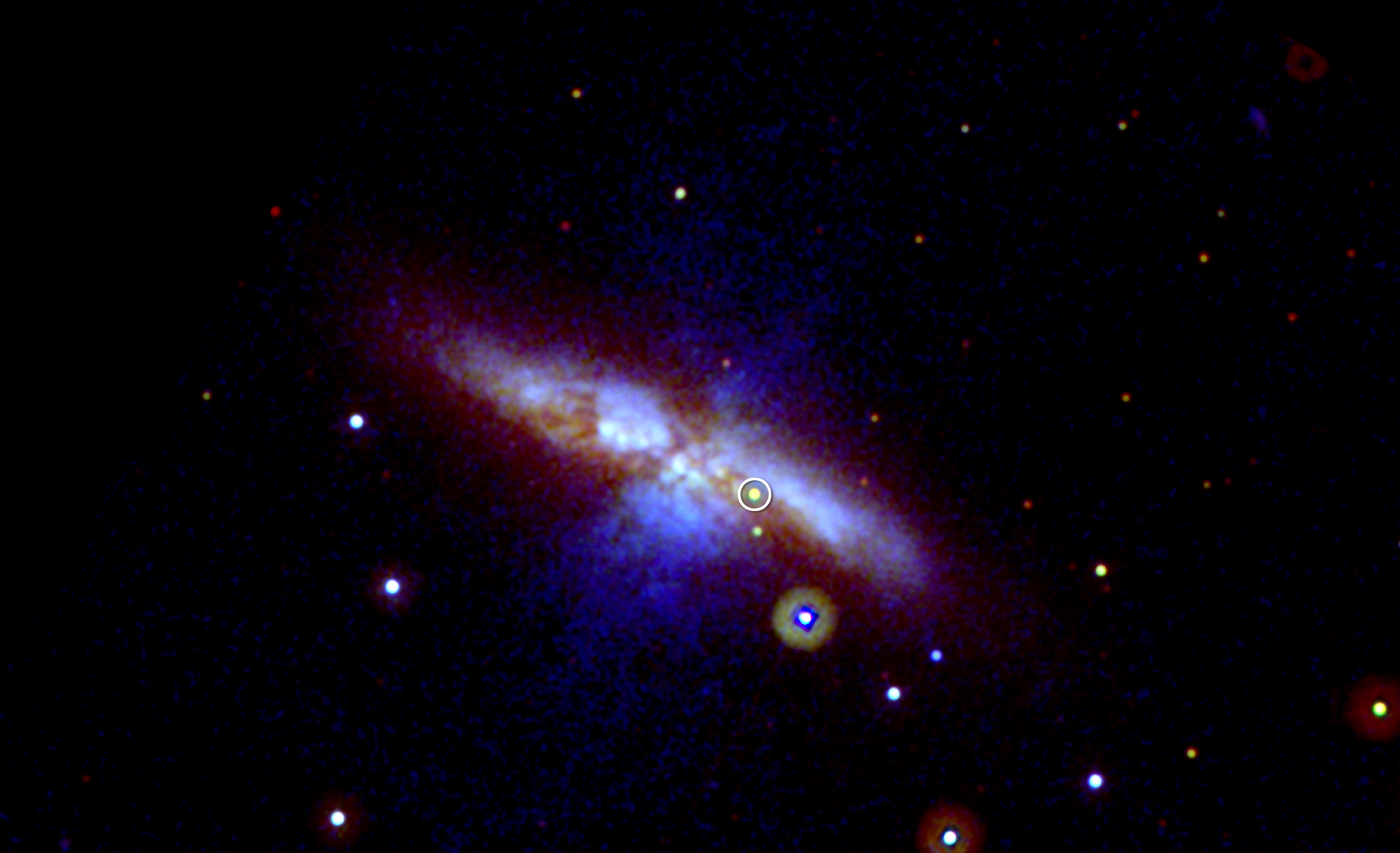
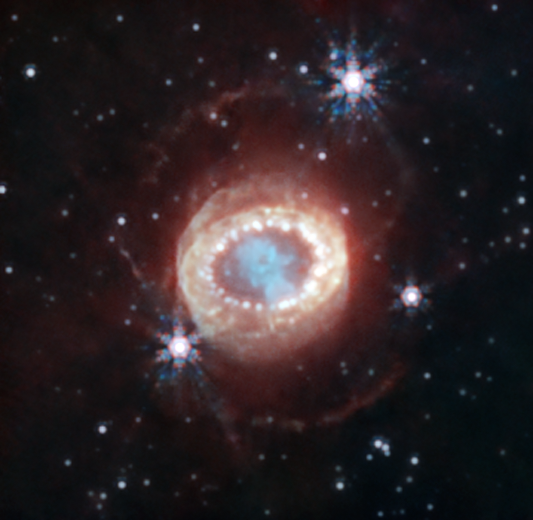
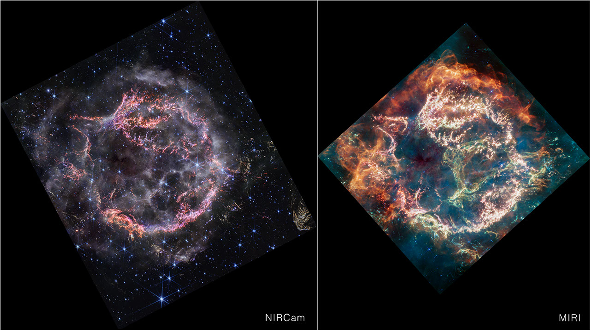
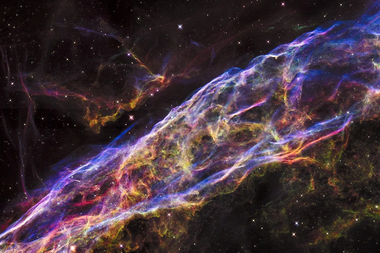
A supernova is observed first as a new point source that brightens and fades over weeks or months. Years later, telescopes may resolve the ejecta and shocks as a remnant. The gallery above deliberately shows both stages.

Ia

Thermonuclear supernova

A carbon–oxygen white dwarf in a binary system undergoes runaway nuclear burning and is disrupted. The light curve is powered principally by the radioactive decay chain 56Ni → 56Co → 56Fe. Type Ia spectra lack hydrogen and show strong silicon near maximum light.

They are standardizable, not perfectly standard: broader, slower-declining light curves are intrinsically brighter, and colour carries luminosity and dust information.

II / Ib / Ic

Core-collapse supernova

A massive star exhausts nuclear fuel, its core collapses, and the outer layers are expelled. SN 1987A, Cassiopeia A, and the Veil Nebula are core-collapse examples included to show the anatomy of ejecta and blast waves—not the Type Ia distance sample used below.

From photons to expansion history

How a supernova enters the Hubble diagram.

  1. 01

    Observe

    Repeated images measure flux versus time in several bands; spectroscopy supplies classification and redshift.

    f(t, λ) → mB, x1, c, z
  2. 02

    Standardize

    Light-curve shape and colour corrections reduce object-to-object luminosity variation.

    mBcorr = mB + αx1 − βc + …
  3. 03

    Infer distance

    The difference between corrected apparent magnitude and standardized absolute magnitude gives distance modulus.

    μ = mcorr − M = 5 log10(dL/Mpc) + 25
  4. 04

    Fit the curve

    The redshift-dependent shape of μ(z), not a sky image, constrains the expansion history and Ωm.

    μ(z) ↔ H(z), Ωm, ΩΛ

Experiment below

After profiling over an unknown magnitude zero-point, how strongly does the redshift-dependent shape of this subset prefer a low-density flat ΛCDM model over an Ωm = 1 matter-only universe?

Interactive analysis

Model, residual, and likelihood workspace

Loading reference data
02

Distance–redshift relation

Hubble diagram

Pantheon+ subsetCurrent modelMatter-only

Observed distance moduli with diagonal uncertainty bars, compared with the selected flat ΛCDM curve and an offset-profiled matter-only curve.

03

Posterior predictive check

Standardized residuals

(μobs − μmodel) / σeff

Included observations are scaled by their effective diagonal uncertainty. The shaded band marks ±1σ and dashed lines mark ±2σ.

Profile best Ωm

—Δχ² = 1 interval: —

Matter-only separation

—Δχ²; diagonal-only diagnostic

Current fit

—χ² / included light curve

Profiled offset

—absorbs H0–magnitude scale

Deceleration parameter

—at z = 0
04

Parameter inference

Profile likelihood in Ωm

Δχ² after profiling ΔM

The orange line is this lab’s diagonal-error subset profile. The blue band marks the published Pantheon+ SNe-only Ωm benchmark.

05

Interpretation

What the calculation says

Waiting for the first analysis run.

Likelihood scope180-row subset; diagonal errors; simple σint; no systematic covariance. Treat Δχ² as an instructional model comparison.

Calculation

Four equations drive the browser analysis.

01

Flat ΛCDM geometry

The luminosity distance is evaluated numerically with ΩΛ = 1 − Ωm and no radiation term.

dL = (1 + z)c/H0 ∫ dz′/E(z′)
02

Effective uncertainty

The released diagonal distance-modulus error is combined with the selected intrinsic scatter.

σ²eff,i = σ²diag,i + σ²int
03

Profiled calibration

At every Ωm, the additive magnitude offset is solved analytically, isolating curve shape from absolute scale.

ΔM̂ = Σwi(μi − μmodel,i) / Σwi
04

Likelihood profile

The interval is the grid crossing at Δχ² = 1 under independent Gaussian diagonal errors.

χ² = Σ[(μi − μmodel,i − ΔM̂)/σeff,i]²

Data used in this browser

180 light curves, selected reproducibly from 1,701.

Official Pantheon+SH0ES release ↗

Columns and selection

The official distance table is sorted by zHD; 180 evenly spaced row indices preserve the full 0.00122–2.26137 redshift span. The source file is checksum-pinned and can be rebuilt with the included acquisition script.

Object identifier
CID
Hubble-frame redshift
zHD
Distance modulus
MU_SH0ES
Diagonal uncertainty
MU_SH0ES_ERR_DIAG
View data JSONImage credits JSON

Numerical scope

  • Default selection: 168/180 rows at z ≥ 0.010.
  • Default scatter: σint = 0.10 mag, added in quadrature.
  • Fit grid: Ωm = 0.05–1.00 in steps of 0.005.
  • Covariance: diagonal terms only; the official systematic covariance is not loaded.
  • Calibration: ΔM is profiled, so this experiment does not independently measure H0.
Inspect all 180 bundled observationsObject, z, μ, uncertainty, inclusion, and residual
ObjectzHDμσdiagIncludedResidualStandardized