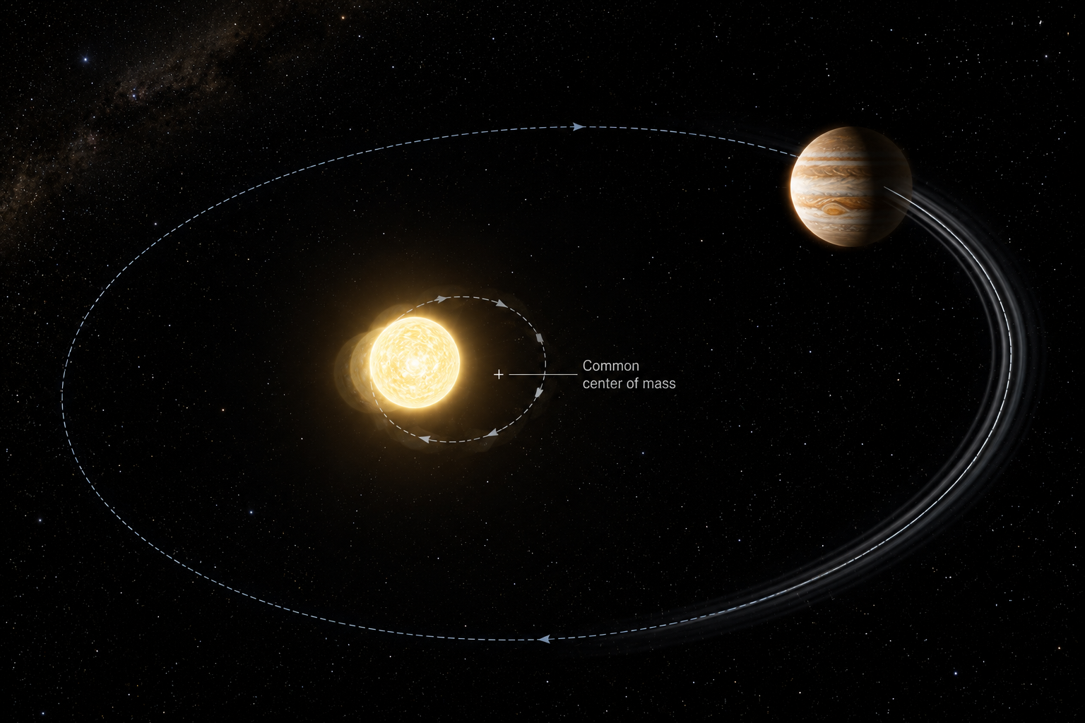
AI-generated artist's concept — not a real photograph. See the report for actual RV spectroscopy data.
The method that found the first exoplanet around a Sun-like star: watch a star's spectral lines shift back and forth as an orbiting planet's gravity tugs it in a small, periodic wobble. This repo works through the physics, solves Kepler's equation and builds the Keplerian RV model from scratch, fits it to a simulated dataset with SciPy's nonlinear least squares and Lomb-Scargle periodogram, and validates the whole pipeline by injecting a known signal and recovering it. **[Open the full report](https://biswajit1999.github.io/radial-velocity-detection-method/)** — the live GitHub Pages version. You can also open `index.html` locally in a browser, or serve it with `python -m http.server` from this directory. Related, from the same author: [Jana's RV Doppler Observatory](https://biswajit1999.github.io/Jana-s-RV-Doppler-Observatory/), an earlier radial-velocity lab covering related Doppler-spectroscopy analysis. ## The physics ### Two bodies orbiting their common center of mass A planet doesn't orbit a fixed star — star and planet both orbit their mutual center of mass (the barycenter), with the star tracing out a much smaller version of the planet's own orbit, scaled down by the mass ratio $M_p/M_\star$. That small stellar orbit is periodically Doppler-shifted toward and away from Earth as seen along our line of sight, imprinted as a tiny periodic shift in the star's absorption-line wavelengths — a shift of order meters per second, measured against light traveling at $3\times10^8$ m/s, which is why this technique depends on extremely high-resolution spectroscopy. ### The semi-amplitude equation, and what each factor means The velocity semi-amplitude of that wobble is: $$K = \left(\frac{2\pi G}{P}\right)^{1/3} \frac{M_p \sin i}{(M_\star + M_p)^{2/3}} \frac{1}{\sqrt{1-e^2}}$$ Reading it term by term: $(2\pi G/P)^{1/3}$ comes from Kepler's third law setting the orbital velocity scale; $M_p \sin i / (M_\star+M_p)^{2/3}$ is the mass ratio that sets how big a wobble the planet induces (in the common limit $M_p \ll M_\star$, this reduces to roughly $M_p \sin i / M_\star^{2/3}$ — the star's own mass suppresses the signal, but only with a 2/3 power, not a square root); and $1/\sqrt{1-e^2}$ boosts $K$ for eccentric orbits, since the star moves fastest at periastron. The $\sin i$ factor is the fundamental limitation: since radial velocity only measures the line-of-sight component of the star's motion, and the orbital inclination $i$ is usually unknown, RV alone gives only a **minimum mass**, $M_p \sin i$, not the true mass — resolvable only with an independent inclination measurement (e.g. from a transit, or astrometry). Jupiter induces about 12.5 m/s on the Sun; Earth induces about 9 cm/s — far below what any instrument can currently measure for an Earth twin around a Sun-like star. ### Why an eccentric orbit isn't just a shifted sine wave For a circular orbit the RV curve is a pure sinusoid. For an eccentric orbit, the star moves faster near periastron and slower near apastron, which distorts the curve into a shape that rises steeply and falls off more gradually (or vice versa, depending on viewing angle) — described by first solving Kepler's equation $M = E - e\sin E$ for the eccentric anomaly $E$ given the mean anomaly $M$ (done here by Newton-Raphson iteration, since it has no closed-form solution), then converting $E$ to the true anomaly $\nu$ before evaluating $K(\cos(\nu+\omega) + e\cos\omega)$. ## Why this method matters Radial velocity was how 51 Pegasi b, the first exoplanet found around a Sun-like star, was discovered in 1995 — and unlike transit photometry, it works regardless of orbital inclination (as long as it's not perfectly face-on) and directly constrains mass rather than radius, making it the essential complement to transit surveys for measuring real planet densities and bulk compositions. Per the NASA Exoplanet Archive's confirmed-planet counts by discovery method (accessed 2026-08-14), radial velocity accounts for 1,197 of 6,336 confirmed exoplanets (~19%) — the second most productive method after transit photometry (4,676, ~74%), ahead of microlensing (282, ~4%) and direct imaging (98, ~2%). Major facilities driving this include HARPS (La Silla, ~1 m/s precision), ESPRESSO (VLT, sub-m/s precision), and Keck/HIRES. **Limitation:** the induced wobble scales as roughly $M_p \sin i / M_\star^{2/3}$ (see the equation above — not a simpler $1/\sqrt{M_\star}$ scaling), and favors massive, close-in planets around bright, quiet, slowly rotating stars. Stellar "jitter" from spots, plages, and granulation (often 1-5 m/s or more) is a fundamental noise floor that no amount of instrumental precision alone can remove. ## What this repo's code does `scripts/radial_velocity_demo.py`: 1. Injects a known Keplerian orbit (period, semi-amplitude K, eccentricity) sampled the way a ground-based spectrograph campaign actually observes — irregular nightly cadence with seasonal observing-window gaps, not a smooth, evenly sampled curve. 2. Adds noise combining HARPS's own published ~1 m/s single-measurement photon-noise precision with a ~1.5 m/s stellar jitter term added in quadrature — both published regimes. 3. Recovers the orbital period from a Lomb-Scargle periodogram (`scipy.signal.lombscargle`), then refines period, K, eccentricity, and argument of periastron with a full Keplerian least-squares fit (`scipy.optimize.curve_fit`) built on a from-scratch Kepler-equation solver and RV model — the periodogram and the nonlinear optimizer themselves are SciPy's, not reimplemented here. 4. Bounds the fit's eccentricity, period, and semi-amplitude directly in the optimizer (not just inside the model function), so the fitted value used for the mass calculation can't come out unphysical even if the search briefly considers points outside the valid range. 5. Converts the recovered K into a minimum mass $M_p \sin i$ using the formula above and a fixed host star mass, and reports the error against the known injected values. Run it yourself: ```bash pip install -r requirements.txt python scripts/radial_velocity_demo.py ``` ## Tests `tests/test_radial_velocity.py` checks the Kepler solver residual, the circular-orbit limit, a mass/K round trip, and — as a regression guard — that minimum mass scales as Mstar^(2/3) at fixed K, not the Mstar^(1/2) scaling an earlier version of this README incorrectly stated. Runs automatically on every push via GitHub Actions; run locally with: ```bash pytest tests/ -v ``` ## Sanity check against a real target's published parameters The K equation applies to the planet that started it all. 51 Pegasi b's real orbital parameters from a single self-consistent study (NASA Exoplanet Archive): period 4.230797 days, minimum mass 0.464 Jupiter masses, host star mass 1.069 Solar masses, eccentricity 0.0042. Feeding these straight into `minimum_mass_mearth`'s underlying formula (inverted here to predict K instead of mass): ``` P = 4.230797 * 86400 s = 365,540 s Mp = 0.464 * 1.898e27 kg = 8.807e26 kg Mstar = 1.069 * 1.989e30 kg = 2.126e30 kg K = (2*pi*G/P)^(1/3) * Mp / (Mstar+Mp)^(2/3) / sqrt(1-e^2) = 55.73 m/s ``` The same study's own measured semi-amplitude is 55.73 m/s — the formula reproduces the published value essentially exactly, because the minimum mass in that study was itself derived from this same K measurement. That circularity is expected and not a weakness: it confirms the equation and the published numbers are internally consistent, which is precisely what you'd want to check before trusting either one on a target where you don't already know the answer. ## Result | Quantity | Injected | Recovered | Error | |---|---|---|---| | Period | 4.23 days | 4.2303 days | 0.01% | | K (semi-amplitude) | 92.0 m/s | 92.00 m/s | 0.01% | | Mp sin i | 235.7 Earth masses | 235.8 Earth masses | 0.00% | With HARPS-class noise and only 60 irregularly sampled nights, the periodogram cleanly and unambiguously identifies the true period, and the phase-folded Keplerian fit recovers the orbit to well under 1% error on every parameter. ## Limitations The injected K (92 m/s) sits at very high signal-to-noise against ~1.8 m/s combined noise, so this is a demonstration that a strong Keplerian signal can be fitted cleanly — not a test of recovery near the noise floor, where real degeneracies between period, eccentricity, and sampling gaps become much harder to break. There's also no false- alarm-probability calculation on the periodogram peak, no fitted instrumental jitter term (jitter is added to the simulated data but not solved for in the fit), and no long-term trend or additional companion in the model — all standard components of a real RV analysis pipeline. ## Extending this To close some of that gap: rerun with K reduced toward the noise floor (a few m/s) and see how the periodogram and fit degrade; add a jitter parameter to the fit itself rather than only to the simulated data, and compare the fitted jitter to the true injected value; compute a bootstrap or analytic false-alarm probability for the periodogram peak instead of just taking the highest one; and try injecting a second, non-interacting planet to see how period aliasing and signal subtraction ("pre-whitening") work in a multi-planet system. Real RV pipelines such as `radvel` and `RadVel`'s underlying MCMC/nested- sampling fitters handle all of this and are worth comparing your own fit against. ## Why this repo uses simulated (not raw archival) data This repo demonstrates the *method itself* — its sensitivity to sampling, noise, and orbital geometry — which is best shown with a known "ground truth" to validate recovery against. This portfolio's companion `*-exoplanet-report` repositories instead each analyze one real target's archival JWST/HST/Spitzer/ground-based spectra directly, with no simulated data. Both approaches are stated plainly here rather than blurring the two. ## Repository structure ```text scripts/radial_velocity_demo.py Keplerian RV model + periodogram + fit + injection-recovery test figures/ generated plot + summary_statistics.csv ``` ## References 1. Mayor, M. and Queloz, D., 1995. A Jupiter-mass companion to a solar-type star. *Nature*, 378, pp.355-359 — the first exoplanet discovered around a Sun-like star (51 Pegasi b). 2. Marcy, G.W. and Butler, R.P., 1998. Detection of Extrasolar Giant Planets. *Annual Review of Astronomy and Astrophysics*, 36, pp.57-97. 3. Lovis, C. and Fischer, D., 2010. Radial Velocity Techniques for Exoplanets, in *Exoplanets*, ed. S. Seager, University of Arizona Press, pp.27-53. 4. Lomb, N.R., 1976. Least-squares frequency analysis of unequally spaced data. *Astrophysics and Space Science*, 39, pp.447-462. 5. Mayor, M. et al., 2003. Setting New Standards with HARPS. *The Messenger*, 114, pp.20-24 — the ~1 m/s instrumental precision used above. 6. Fulton, B.J. et al., 2018. RadVel: The Radial Velocity Modeling Toolkit. *Publications of the Astronomical Society of the Pacific*, 130(986), 044504 — the `radvel` package referenced above. 7. NASA Exoplanet Archive,