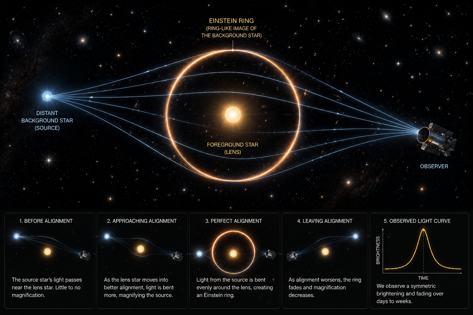
AI-generated artist's concept — not a real photograph. See the report for the real physics and detection statistics.
The only technique sensitive to planets at wide separations, low-mass planets around faint or distant stars, and free-floating planets with no host star at all: a foreground star's gravity briefly bends and magnifies the light of a background star it passes in front of, and a planet orbiting that foreground "lens" star can add a short, sharp perturbation on top of the smooth main brightening. This repo works through the physics, implements a point-source point-lens (PSPL) model and the standard planetary-perturbation scaling relations in Python, and detects a simulated perturbation without ever telling the search code where or how large it is. **[Open the full report](https://biswajit1999.github.io/gravitational-microlensing-detection-method/)** — the live GitHub Pages version. You can also open `index.html` locally in a browser, or serve it with `python -m http.server` from this directory. ## The physics ### Why light bends and brightens General relativity says mass curves spacetime, and light follows that curvature. When a foreground "lens" star passes close to our line of sight to a background "source" star, it bends the source's light into two separate images that we can't resolve individually — instead we see their combined, magnified brightness. The characteristic angular scale of this bending is the Einstein radius: $$\theta_E = \sqrt{\frac{4GM_L}{c^2}\left(\frac{1}{D_L} - \frac{1}{D_S}\right)}$$ where $M_L$ is the lens mass and $D_L$, $D_S$ are the observer-lens and observer-source distances. For a typical Galactic lens this works out to roughly a milliarcsecond — far too small to resolve directly, which is why microlensing is detected purely through the brightness change, not by imaging anything. ### The single-lens light curve For a single point-mass lens, the total magnification as a function of the source-lens angular separation $u$ (in units of $\theta_E$) is: $$A(u) = \frac{u^2+2}{u\sqrt{u^2+4}}, \qquad u(t) = \sqrt{u_0^2 + \left(\frac{t-t_0}{t_E}\right)^2}$$ $u_0$ is the minimum impact parameter (how close the alignment gets, in Einstein radii), $t_0$ the time of closest approach, and $t_E = \theta_E / \mu_{rel}$ the Einstein-radius crossing time — the lens-source relative proper motion sets how long the whole event takes, typically days to weeks for stars toward the Galactic bulge. Plugging in $u_0 \to 0$ shows the magnification formally diverges for a true point source passing exactly behind the lens; real events are capped by the source star's own finite angular size. ### What a planet adds If the lens star hosts a planet, the planet's own much smaller field perturbs the light bending near its position, producing a brief deviation from the smooth single-lens curve — sometimes a spike, sometimes a dip, depending on the source's trajectory relative to the planet's caustic. The perturbation's characteristic duration scales with the star-planet mass ratio $q = M_p/M_\star$ roughly as $t_{pert} \sim t_E\sqrt{q}$ (Mao & Paczynski 1991; Gould & Loeb 1992). Its amplitude is more sensitive to the details — source trajectory, caustic topology, and how close the source passes to the planet's caustic all matter, so $\delta A/A \sim \sqrt{q}$ is a rough, order-of- magnitude scaling rather than a fixed relationship. What's robust is the duration scaling: even a Jupiter-Sun mass ratio of order $10^{-3}$ gives a perturbation lasting only $\sim\sqrt{q} \approx 3\%$ of the main event's duration — hours out of weeks — which is why real microlensing surveys need high-cadence, round-the-clock coverage to catch planetary signals at all. ## Why this method matters Microlensing needs no light at all from the planet, and its sensitivity peaks for planets a few Einstein radii from their star — the "cold" region beyond the ice line that transit and (to a lesser extent) radial velocity struggle to probe. It's the leading method for finding low-mass planets at Jupiter-to-Neptune-like separations around typical Milky Way stars, and the only method capable of finding free-floating, unbound planets with no detectable host at all. Ground-based surveys (OGLE, MOA, KMTNet) monitor hundreds of millions of bulge stars every night looking for these events, and NASA's Roman Space Telescope (currently targeting launch by 30 August 2026) is purpose-built to run a large-scale space-based microlensing survey with far better cadence and precision. Per the NASA Exoplanet Archive's confirmed-planet counts by discovery method (accessed 2026-08-14), microlensing accounts for 282 of 6,336 confirmed exoplanets (~4%) — third by count after transit (4,676, ~74%) and radial velocity (1,197, ~19%), ahead of direct imaging (98, ~2%), but disproportionately important for demographics the other methods can't reach: cold, wide-separation planets around typical Milky Way stars, and free-floating planets with no bound host at all. **Limitation:** every microlensing event is a one-time, non-repeating alignment between three objects (observer, lens, source) — once it's over, it's over, and the lens star usually can't be reobserved or characterized in detail afterward. Planet parameters derived from a single event carry real, often irreducible degeneracies (particularly the lens system's distance and total mass) that need additional follow-up, such as high-resolution imaging years later once the lens and source have separated on the sky, to fully resolve. ## What this repo's code does `scripts/microlensing_demo.py` builds a simulated light curve, then detects and characterizes the planetary signal in it without any step of the analysis referencing the values used to generate it: 1. **Simulate.** Build a PSPL magnification event with an Einstein time and impact parameter, sampled at high-cadence survey rates (KMTNet-class, every 30 minutes) with a ~2% ground-based crowded- field photometric noise level, and add a short planetary perturbation using the amplitude/duration scaling relations above (an analytic approximation, not a full inverse-ray-shooting binary-lens computation — see Limitations). 2. **First-pass fit.** Fit the single-lens model to the *entire* light curve, seeded only from what the data itself shows: the peak time, an impact-parameter estimate from the peak magnification via the small-$u$ approximation $A(u)\approx 1/u$, and a timescale estimate from the light curve's width at half maximum. 3. **Detect.** Flag points that deviate from that fit by more than a noise threshold, and take the longest contiguous run of flagged points as the perturbation window — the search never looks at the time or mass ratio used to inject the signal. 4. **Re-fit clean.** Mask the detected window and re-fit the single-lens model on the remaining points, so the baseline isn't biased by the planetary signal. 5. **Characterize.** Fit a Gaussian bump to the residual inside the detected window, seeded from the window's own center and width, then invert its fitted amplitude and duration through the scaling relations for two estimates of the mass ratio $q$, combined as their geometric mean. These two numbers are not statistically independent checks on each other — both come from the same single Gaussian fit, so they share its fitting errors rather than providing two separate pieces of evidence. Run it yourself: ```bash pip install -r requirements.txt python scripts/microlensing_demo.py ``` ## Tests `tests/test_microlensing.py` checks the PSPL magnification formula against its closed-form solution and, more importantly, verifies the perturbation-window detector on synthetic residuals it hasn't seen the injection parameters for — including a check that pure noise (no injected bump) correctly returns no detection. Runs automatically on every push via GitHub Actions; run locally with: ```bash pytest tests/ -v ``` ## Sanity check against a real target's published parameters OGLE-2005-BLG-390Lb, the first cold super-Earth found by microlensing (Beaulieu et al. 2006), gives a real mass ratio to check the scaling relations against. Its published planet and host-star masses: 5.5 Earth masses, orbiting a ~0.22 Solar-mass M dwarf. ``` Mp = 5.5 * 5.972e24 kg = 3.285e25 kg Mstar = 0.22 * 1.989e30 kg = 4.376e29 kg q = Mp / Mstar = 7.5e-5 ``` A mass ratio of order $10^{-4}$–$10^{-5}$ like this one predicts, via $t_{pert} \sim t_E\sqrt{q}$, a perturbation lasting only about 1% of the event's total Einstein time — for a typical bulge event with $t_E$ of a few weeks, that's a perturbation measured in hours, exactly why real microlensing planet searches need continuous, high-cadence monitoring from multiple longitudes (OGLE, MOA, and KMTNet operate telescopes spread across the globe partly for this reason: a few-hour anomaly is easy to miss entirely from a single site with one clear-weather window per night). ## Result | Quantity | Injected | Recovered | Error | |---|---|---|---| | Perturbation window | centered at 22.0 days | detected at [21.48, 22.60] days | — | | Einstein time (tE) | 20.0 days | 20.010 days | 0.05% | | Mass ratio (q) | 1.50×10⁻³ | 1.48×10⁻³ | 1.07% | The detection step finds the perturbation window from the residuals alone and lands within about half a day of where it was actually injected; the single-lens fit recovers the event timescale cleanly, and the mass ratio comes out within about 1% — worse than a fit that was handed the answer in advance would report, and a more meaningful number because of that. ## Limitations This repo's planetary-perturbation model uses the scaling relations for characteristic amplitude and duration, not a full binary-lens computation (which requires solving a 5th-order complex polynomial for image positions via inverse ray-shooting or contour integration). This is a standard back-of-the-envelope approach for a rough mass-ratio estimate, but a published microlensing planet detection fits the full binary-lens light curve in detail, which is also needed to break the mass-distance degeneracy mentioned above. The detection step here also uses a simple sigma-threshold flag on a single light curve; real surveys combine detection statistics across a network of telescopes and correct for finite-source effects near the caustic, which this simulation doesn't model. ## Extending this A natural next step if you want to go further than the scaling-relation approximation here: implement the full binary-lens magnification map by solving for image positions at each source position (the lens equation becomes a complex polynomial of degree 5 in the image plane), or use an existing package such as `MulensModel` or `pyLIMA`, both of which implement real binary-lens fitting used in published microlensing papers, and fit this repo's simulated light curve with one of them to see how much the mass-ratio estimate changes. ## Why this repo uses simulated (not raw archival) data This repo demonstrates the *method itself* — how a planetary signal gets found and measured, and where the approximations break down — which is best shown with a known "ground truth" to check the detection against. This portfolio's companion `*-exoplanet-report` repositories instead each analyze one real target's archival JWST/HST/Spitzer/ ground-based spectra directly, with no simulated data. Both approaches are stated plainly here rather than blurring the two. ## Repository structure ```text scripts/microlensing_demo.py PSPL model + blind detection + mass-ratio recovery figures/ generated plot + summary_statistics.csv ``` ## References 1. Mao, S. and Paczynski, B., 1991. Gravitational microlensing by double stars and planetary systems. *The Astrophysical Journal Letters*, 374, L37. 2. Gould, A. and Loeb, A., 1992. Discovering planetary systems through gravitational microlenses. *The Astrophysical Journal*, 396, pp.104-114. 3. Bond, I.A. et al., 2004. OGLE 2003-BLG-235/MOA 2003-BLG-53: A Planetary Microlensing Event. *The Astrophysical Journal Letters*, 606(2), L155 — the first microlensing planet detection. 4. Gaudi, B.S., 2012. Microlensing Surveys for Exoplanets. *Annual Review of Astronomy and Astrophysics*, 50, pp.411-453. 5. Spergel, D. et al., 2015. Wide-Field InfraRed Survey Telescope- Astrophysics Focused Telescope Assets (WFIRST-AFTA) 2015 Report, arXiv:1503.03757 — design study for the Roman Space Telescope's microlensing survey. 6. Poleski, R. and Yee, J.C., 2019. Modeling microlensing events with MulensModel. *Astronomy and Computing*, 26, pp.35-49 — the `MulensModel` package referenced above. 7. NASA Exoplanet Archive,