Exploration · Evidence · A deeper universe

Dark Matter
Evidence Lab

Investigating invisible mass through galaxy rotation curves, gravitational lensing, clusters and cosmology.

175SPARC galaxies
3,391resolved velocities
4evidence scales

Start here

In simple words

You do not need a cosmology textbook to enter the project. These two ideas are related only because both are still physically unexplained.

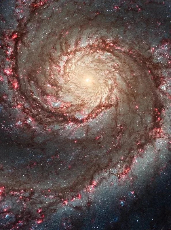
Hubble image of the Whirlpool Galaxy M51.
Dark matter

Mass we cannot see with light.

Galaxies and clusters behave as if extra gravitating mass is present. We infer it from motion, lensing and cosmic structure—but we still do not know what it is made of.

We can measure
its gravitational effects
We still do not know
its microscopic identity
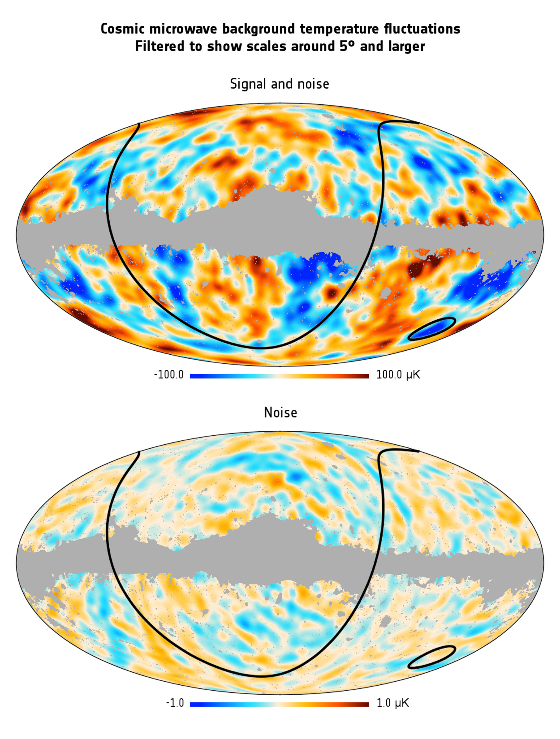
Planck all-sky view of the cosmic microwave background.
Dark energy

The name for accelerated cosmic expansion.

The universe is not only expanding; its expansion is accelerating. Dark energy is the label for whatever drives that late-time behaviour in our models.

We can measure
the expansion history
We still do not know
the underlying physics

The universe today

A cosmic inventory

In a Planck-like base flat ΛCDM reference model, ordinary matter is only a small fraction of the total cosmic energy budget.

See how the percentages are calculated →
Radiation0.01%photons + relativistic speciessource + maths
Ordinary matter4.9%atoms, gas and starssource + maths
Cold dark matter26.4%gravitating componentsource + maths
Dark energy68.7%late-time expansion termsource + maths
Today · a = 1Reference: base flat ΛCDM · Planck 2018 parameter baseline
Why do the fractions change with cosmic time?

H²(a) = H₀² [ Ωra−4 + Ωma−3 + Ωka−2 + ΩΛ ]

Radiation dilutes fastest; matter follows volume; a cosmological constant remains constant. The quantitative cosmology laboratory later in the page lets you move through this history.

Key areas

From evidence to new possibilities

Four visual entry points into the project. Each opens into a quantitative section below.

The research frontier

A fundamental question remains.

We can map where unseen gravity acts. We can constrain how the dark component behaves. We still do not know what it is—and that is precisely where the open research begins.

Explore the open questions
How do scientists infer something they cannot see?Open the observation → inference primer

03

How can we see something dark?

Follow the transformation, not the metaphor

Each arrow changes the epistemic status of the information. Assumptions are part of the result, not footnotes to hide.

  1. ObservedPhotonsinstrument response · calibration
  2. MeasuredPosition / spectrumastrometry · spectroscopy
  3. DerivedKinematics / distortiongeometry · redshift · PSF model
  4. InferredGravitational fielddynamical equilibrium · gravity law
  5. ModelledMass distributionsymmetry · priors · nuisance parameters
  6. HypothesisMicroscopic identityinteraction model · independent experiment

Photons locate light. Motion probes gravity. Lensing maps projected mass. Cosmology tests content and history. Detectors search for microscopic interactions.

Galaxies175 SPARC systems · 3,391 velocities
ClustersLensing mass versus hot gas
CosmosStructure imprinted on the CMB
LaboratoryRare-event particle searches

Observatory context · directly credited

One hypothesis, independent scales

Dark matter is inferred through different measurements. These credited images are context—not substitutes for the quantitative data below.

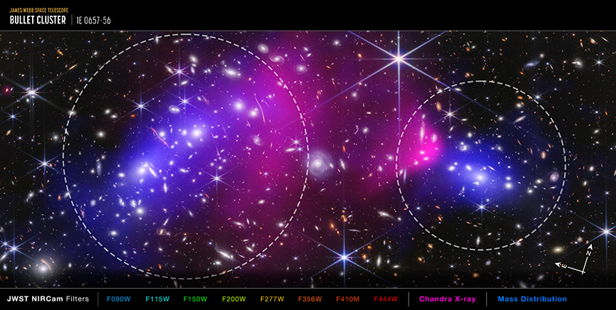
Webb and Chandra composite of the Bullet Cluster, with pink X-ray gas and blue gravitational-lensing mass maps separated across the collision.
Merging cluster · lensing + X-ray Bullet Cluster: mass and hot gas separate

Blue maps the lensing-derived mass distribution; pink maps X-ray-emitting gas. Dashed circles locate the two colliding galaxy clusters.

Credit: X-ray NASA/CXC/SAO · NIR NASA/ESA/CSA/STScI · processing NASA/STScI/J. DePasquale
Hubble image of the face-on Whirlpool Galaxy M51, showing its bright core, dust lanes and spiral arms.
Galaxy · visible structure M51 through Hubble

A real spiral galaxy used as visual context. The selectable rotation curves below come from the SPARC catalogue, not this photograph.

Credit: NASA, ESA, S. Beckwith (STScI) and Hubble Heritage Team (STScI/AURA)
Planck all-sky maps comparing large-scale cosmic microwave background temperature signal plus noise with instrument noise.
Cosmology · early universe Planck’s microwave sky

Temperature fluctuations constrain the universe’s matter content and the growth conditions for later cosmic structure.

Credit: ESA/Planck Collaboration
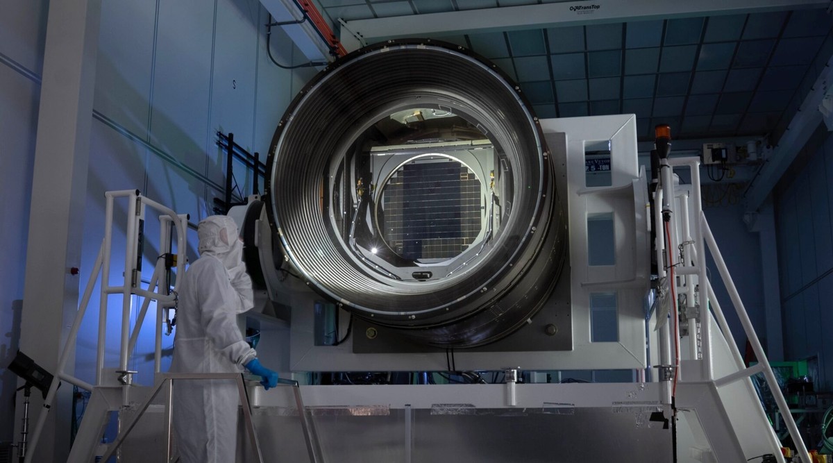
Real photograph of Rubin Observatory's LSST Camera in a cleanroom, with a technician standing beside its large front opening.
Technology · wide-field survey Rubin’s 3.2-gigapixel eye

Wide, repeated imaging lets researchers map enormous galaxy populations and test small gravitational distortions statistically.

Credit: Olivier Bonin/SLAC National Accelerator Laboratory

Every image is a real mission or observatory product. Full credits and primary-source links appear directly on each image.

Interactive galaxy workbench

Compare published rotation curves, one system at a time

The same transparent model is applied across spirals and gas-rich dwarfs. A fit describes gravitational evidence; it does not identify a particle.

Guided evidence sequence

Build the inference one layer at a time

Lab mode shows every available measured, modelled and inferred layer.

Observation → model

Rotation-curve decomposition

The rotation-curve plot is loading.

Diagnostic

Standardised residuals

(observed − model) / σ

Residual diagnostics are loading.

Parameter response

Δχ² surface

velocity × scale radius

Likelihood surface is loading.

Fit telemetry

Current model

run —

Audit trail

Observed values, model and provenance

Open SPARC source
Show the accessible data table
Observed rotation curve and current model evaluation
Radius (kpc) Observed (km/s) σ (km/s) Gas (km/s) Disc, scaled (km/s) Halo (km/s) Total (km/s) Residual / σ
Dataset—
Distance—
Upstream SHA-256—
TransformParsing and column renaming only

Phase 3–4 · galaxies as a population

Population and acceleration-relation laboratory

Filter one shared population and compare a global baryonic scaling relation with all resolved acceleration measurements. Correlation is evidence for a regularity—not, by itself, a microscopic explanation.

Observed + assumed M/L

Baryonic Tully–Fisher plane

Vflat versus Mbar

The population plot is loading.

Phenomenological comparison

Radial acceleration relation

gbar versus gobs

The acceleration-relation plot is loading.

Show selection, equations and accessible filtered catalogue

BTFR: Mbar = 0.5 L3.6 + 1.33 MHI. Galaxies without a published positive Vflat are excluded from that panel. The stellar mass-to-light ratio is an explicit fixed assumption, not a measurement.

RAR: gobs = Vobs²/R and gbar = (Vgas|Vgas| + 0.5Vdisk² + 0.7Vbulge²)/R. The reference curve uses g† = 1.2 × 10⁻¹⁰ m s−2. Non-positive derived accelerations are excluded; distance and inclination systematics are not propagated here.

Subsets: low/high surface brightness split at the catalogue median effective surface brightness; gas dominated means the stored fixed-M/L gas fraction exceeds 0.5. Quality flags are SPARC’s own: 1 high, 2 medium, 3 low.

Filtered SPARC galaxy population
GalaxyTypeQDistance (Mpc)Inclination (deg)SBeff (L☉/pc²)Gas fractionVflat (km/s)N
Population data are loading.
Model-dependent inference

These views reproduce relationships within the selected assumptions. They do not establish whether the regularities arise from dark matter, baryonic physics, modified dynamics, selection effects, or a combination.

SPARC data and primary references

Phase E · challenge the model

Alternative dynamics under explicit assumptions

Compare the selected halo configuration with baryons alone and two acceleration-based phenomenological relationships. This tests predictions; it does not declare a winning theory.

1.2 × 10⁻¹⁰ m/s²
0.5 M☉/L☉

Bulge M/L is fixed at 0.7. The acceleration scale and disc M/L are displayed assumptions, not automatically fitted values. Distance, inclination, external-field effects and covariance are omitted.

Model comparison

Velocity predictions

same observed radii

Alternative-model velocity comparison is loading.

Diagnostic

Standardised residual structure

(observed − predicted) / σ

Alternative-model residual comparison is loading.

Established observation

What is measured

Radius, circular velocity, random velocity uncertainty and photometric/gas contributions from SPARC.

Model-dependent inference

What is assumed

Stellar mass-to-light ratios, axisymmetric circular motion and the selected functional relationship between baryonic and observed acceleration.

Discriminating evidence

What would help

Independent distance and inclination constraints, vertical dynamics, lensing, satellites, clusters and cosmology test whether one galaxy-scale relation generalises.

Show equations and accessible comparison table

Empirical RAR: gpred = gbar / [1 − exp(−√(gbar/g†))]. It compactly describes a galaxy-scale regularity but is not itself a microscopic theory.

Simple ν: gpred = [½ + √(¼ + a₀/gbar)]gbar. This is a MOND-like phenomenological interpolation; relativistic completion and external-field assumptions are outside this calculation.

Comparison: χ² values use only quoted independent random velocity errors. Lower residuals under these settings do not establish physical truth or account for model flexibility and systematics.

Alternative-dynamics comparison at each measured radius
Radius (kpc)ObservedσBaryonicPhenomenologicalCurrent haloPhen. residual/σHalo residual/σ
Comparison data are loading.

Phase F · clusters as gravitational laboratories

Quantitative lensing and colliding-cluster laboratory

Change the lens geometry, reveal each measured tracer and test why a separation between hot gas, galaxies and reconstructed total mass is informative.

1.00
1,150 km/s
Evidence layers

Flat ΛCDM geometry: H₀ = 70 km/s/Mpc, Ωm = 0.3. The velocity dispersion sets an illustrative singular-isothermal-sphere scale; it is not a fit to the displayed image.

Derived reconstruction

Cluster layer map

GalaxyX-ray gasTotal mass

Cluster reconstruction is loading.

Schematic, not a dark-matter photograph. Lensing contours represent a model-dependent inversion of many background-galaxy shapes; the gas layer represents an X-ray tracer.

Observed tracer

What telescopes measure

Optical images locate galaxies, X-ray photons trace hot plasma and coherent distortions appear in background-galaxy shapes.

Reconstructed quantity

What lensing infers

Shape distortions constrain projected gravitational potential. Recovering a convergence or mass map requires source redshifts, calibration and inversion assumptions.

Discriminating pattern

Why collisions matter

Gas experiences ram pressure; stars are nearly collisionless. When most reconstructed mass follows galaxies instead of gas, the dominant gravitating component is not the plasma.

Show calculation contract and accessible system table

Critical density: Σcrit = c²Ds/(4πG DlDls). A lower value means the chosen lens–source geometry is more efficient.

SIS scale: θE = 4π(σv/c)²Dls/Ds. This compact proxy connects velocity dispersion to angular lens strength; real merging clusters require multi-component mass models.

Inference limit: Lensing responds to projected total gravity. Calling the residual component “dark matter” combines that map with baryonic tracers and a gravity model.

Cluster systems and live lens-geometry calculations
SystemLens zSource zkpc/arcsecΣcrit (M☉/pc²)θE (arcsec)Evidence status
Cluster data are loading.

Phase G · early universe to experiments

Cosmology, candidate and experiment landscape

Connect the cosmic matter budget to the very different instruments that test candidate particles, fields and compact objects. Null results constrain models; they are not evidence that dark matter is absent.

0.00
Advanced cosmology parameters Ω, w₀–wₐ, H₀ and BAO redshift
0.049
0.264
−1.00
0.00
67.4 km/s/Mpc
0.80

This explorer preserves spatial flatness at the present epoch and uses the CPL form w(a)=w₀+wₐ(1−a). It calculates background expansion and distance response only; it does not compute CMB spectra, run a Boltzmann solver, or evaluate Planck/DESI likelihoods.

Calculated background

Component fractions through expansion

radiation · baryons · cold dark matter · dark energy

Cosmological component evolution is loading.

Model response · not a DESI likelihood

BAO distance coordinates

D_M/r_d · D_H/r_d

BAO distance response is loading.

ModelH²(a) / H₀²

Radiation ∝ a⁻⁴, matter ∝ a⁻³, curvature ∝ a⁻², and the selected dark-energy response supplies the remaining background term.

What the sliders changeGeometry, growth background and distance response

Ω values alter the component budget; w₀–wₐ changes the dark-energy density history; H₀ rescales the distance ladder; BAO redshift selects the comparison point.

ProvenancePlanck-like reference, not a likelihood rerun

The browser evaluates background equations only. It does not recompute CMB spectra, DESI likelihoods or Boltzmann transfer functions.

Open the percentage mathematics →
Open deeper cosmology interpretation
Independent baryon anchor

Why “all matter is baryonic” fails

Primordial nucleosynthesis and CMB acoustic structure constrain the baryon density. Replacing Ωcdm with baryons changes photon–baryon oscillations instead of reproducing the same sky.

Growth mechanism

Why early clustering matters

Before recombination, baryons are coupled to photons. A non-baryonic component can begin building gravitational wells without participating in that acoustic fluid.

DESI · updated July 2026

Evolving dark energy remains an open test

DESI DR2 full-shape Lyα measurements moved toward the Planck ΛCDM prediction. The site therefore treats w₀–wₐ exploration as a competing-model exercise, not a discovery of evolving dark energy.

DESI Collaboration context
Inference boundary

What cosmology does not identify

A fitted Ωcdm quantifies a gravitating component within a model. It does not specify mass, spin, couplings or a laboratory detection channel.

Candidate atlas

No single search covers “dark matter”

Show experiment landscape and quantitative assumptions
Complementary dark-matter search channels; status as recorded 28 September 2026
ProgrammeChannelObservableClassCurrent result/statusUpdatedSource
Experiment records are loading.

Phase C · Bayesian inference

Posterior workspace

Set explicit uniform priors, run four deterministic Metropolis chains and inspect credible intervals and convergence before interpreting a fitted halo.

Uniform prior bounds

minimum → maximum
Disc M/L
Halo velocity (km/s)
Scale radius (kpc)

4 chains × 2,600 iterations; 1,000 warm-up iterations; thinning 3; deterministic seed 20260927. Priors are uniform within the displayed bounds. The sampler first locates the grid minimum, then adapts proposal widths during warm-up.

Posterior not run for this galaxy and halo model.
Monte Carlo viewRun the chains to populate covariance, trace mixing and autocorrelation. The diagnostic plots below are deliberately compact and linked to the same samples.

Run posterior chains to create marginal distributions and a halo-parameter covariance plot.

Chain traces

Run posterior chains to inspect trace mixing.

Autocorrelation

Run posterior chains to inspect autocorrelation.

Model-dependent inference

The rotation plot gains a 68% posterior predictive interval after sampling. It combines fitted-parameter uncertainty with the quoted SPARC random velocity errors. The current distance and inclination sensitivity settings are held fixed rather than marginalised, and correlated systematics remain outside this browser model. A posterior-predictive p-value near 0 or 1 can flag mismatch; it is not the probability that a halo model is true.

Show accessible posterior summary table
Posterior medians, 68% credible intervals and convergence diagnostics
Parameter16th percentileMedian84th percentileSplit R-hatESS
No posterior samples yet.
Show accessible posterior predictive intervals
Observed velocities, latent model intervals and replicated-observation intervals in kilometres per second
Radius (kpc)ObservedModel q16Model medianModel q84Predictive q16Predictive q84
No posterior predictive intervals yet.

Phase H · scales, frontiers and constrained futures

From subnuclear interactions to the cosmic web

Explore what changes with physical scale, calculate a deliberately simplified encounter rate and distinguish active engineering from conditional or speculative future capability.

01 · observed Measured signal

Recoil, lensing shear, conversion photon, timing shift or another calibrated observable.

02 · derived Physical reconstruction

Instrument calibration and a stated model transform the raw signal into a mass, field or event-rate constraint.

03 · discovery gate Microscopic identity

A reproducible interaction must establish mass, coupling and consistency with the astrophysical abundance.

04 · new-physics gate Control and capture

Detection is not enough: useful engineering requires controllable production, capture, confinement or state manipulation.

05 · conditional Engineering

Only then can sensing, communication, energy or propulsion be evaluated with ordinary conservation laws.

10¹⁹ m
Galactic halo

Which density profile and phase-space distribution fit multiple tracers?

Dynamics, streams, microlensing and lensing

06

If the microscopic physics became controllable

What could humanity actually try to build?

These are conditional engineering studies, not predictions. The images are generated concept art used to visualise the engineering questions—not observational evidence and not a claim that these devices exist. Each idea starts from an explicit physics gate that current evidence has not yet crossed.

Generated concept artwork showing a network of instruments mapping a dark-matter wind around Earth and the Moon.
conditional · closest to present experiments

Direct local sensing

If a reproducible non-gravitational interaction exists, directional detectors could map the local dark-matter velocity field rather than only count events.

Author perspective →
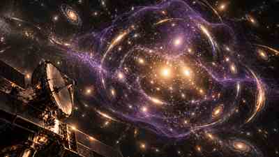
Generated concept artwork of a galaxy cluster lensing field and reconstructed unseen mass distribution.
evidence-grounded

Gravitational environment mapping

Lensing, streams and precision dynamics already let us map unseen gravitating structure without identifying a particle.

Author perspective →
Generated concept artwork showing hypothetical weakly interacting signals linking distant observatories and planetary systems.
speculative

Dark-sector communication

A weakly interacting messenger could penetrate ordinary matter, but the same weak coupling makes generation and detection extraordinarily difficult.

Author perspective →
Generated concept artwork combining a spacecraft, precision observations and a navigation data pipeline.
conditional

Precision inertial navigation

Future field or stream sensors could become an independent reference for local gravitational structure if a stable directional signal were ever demonstrated.

Author perspective →
Generated concept artwork of a field-energy transducer used to illustrate an upper-bound dark-sector energy thought experiment.
upper-bound exercise

Energy extraction limits

Ambient density provides a mass-flux ceiling, but usable power collapses unless capture and conversion physics exist at practical efficiencies.

Author perspective →
Generated concept artwork of an advanced orbital research apparatus used to illustrate a conditional momentum-transfer propulsion experiment.
not supported by current evidence

Propulsion thought experiment

Any engine must transfer directed momentum and close a complete mass, power and heat ledger. Reactionless thrust is not implied by dark matter.

Author perspective →
Open the quantitative futures lab encounter rate · capture · energy · momentum

Encounter-rate sandbox

2.0
−46
0.40
50%

Fixed speed: 220 km/s. The displayed count treats every kilogram as free nucleons with one cross section. It omits nuclear coherence, form factors, thresholds, velocity distribution, shielding and backgrounds, so it is a scaling exercise—not an experiment forecast.

Model boundary

Illustrative contact scale only

A real exclusion or sensitivity curve must specify an interaction operator, target response, detector exposure and statistical treatment.

Hypothesis laboratory

Is dark matter hidden in another dimension?

No extra spatial dimension is required for matter to be electromagnetically dark. A particle in ordinary 3+1-dimensional spacetime can simply lack a useful electromagnetic coupling. Extra-dimensional models are separate, testable beyond-Standard-Model hypotheses.

baseline physics

3 spatial dimensions + time

Weak or absent electromagnetic coupling is enough to prevent ordinary imaging. Gravity can still reveal the mass distribution.

ordinary spacetimephotonsdark stategravity
hypothesis

3+1+n dimensions

Kaluza–Klein, braneworld or bulk-state scenarios can introduce additional states or mediators, but must earn their place through observable deviations—not visual intuition.

visible branecompact/bulk dimensionhypothetical statetestable signature?
Discriminating question

What measurement would tell the scenarios apart?

Collider spectra, modified force laws, missing-energy signatures or other model-specific observables must differ from an ordinary weakly coupled dark sector. “We cannot see it” alone is not evidence for extra dimensions.

Particle Data Group reviews

Discovery-dependent engineering

Could dark matter power or propel a spacecraft?

Only after specifying interaction, capture, energy transfer and momentum transfer. This calculator makes the missing physics explicit and treats a failed engine as a useful result.

identity known?→ coupling?→ controllable?→ capture?→ energy transfer?→ directed momentum?→ engineering

Assumption ledger

10⁶ m²
10⁵ kg
10³⁰ cm⁻²
100%
100%
1.00

Cross section and local density are inherited from the encounter sandbox above. The target column is a deliberately simplified optical-depth proxy. No known material can be assumed to capture dark matter with the selected efficiencies.

Engine feasibility calculation is loading.

Research Frontier

What is known, unknown and decisive

Show technology horizons and falsification gates
Physics-constrained capability horizons, not discovery promises
HorizonPossible capabilityValidation gateConfidence
Research-frontier data are loading.

Phase I · evidence architecture

Trace every claim from observation to inference

Select a node to inspect what it claims, where it comes from and what can break the inference. Arrows are relationships, not proof.

Educator view

Start with the observation nodes, then follow their equations to an inference. The final “microscopic identity” node remains a hypothesis because gravity alone cannot tell us which candidate exists.

Show the complete edge list and reproducibility state
Directed evidence relationships
FromRelationshipTo
Evidence graph is loading.
Reproducible workspace stateExport the current galaxy, halo, cluster, cosmology, future-sandbox and view-mode settings.

Author perspective · long-horizon synthesis

Six deeper essays behind the laboratory

These pages separate my interpretation from the measured evidence. They are first-person scientific reflections, not claims that unresolved physics has been solved.

Capability roadmap · 2026–2076

What the next 50 years can actually improve

This is a staged research pathway, not a promise that discovery will arrive on a schedule. Each stage has a measurable validation gate.

  1. 2026–2035

    Join the sky surveys

    Cross-calibrate Rubin, Euclid and Roman lensing maps; expand resolved galaxy dynamics; keep tonne-scale rare-event detectors accumulating exposure.

    Gate: consistent halo structure across instruments, wavelengths and analysis pipelines.
  2. 2035–2050

    Turn backgrounds into measurements

    Scale ultra-low-background detectors, directional recoil sensing, cryogenic thresholds and axion-band coverage while combining CMB lensing with galaxy surveys.

    Gate: a repeatable signal with target, direction or annual-modulation tests—or stronger exclusions that retire model families.
  3. 2050–2076

    Build for the surviving parameter space

    Condition future observatories on what earlier null results leave open: quantum sensors, interferometric concepts, distributed timing and next-generation underground targets.

    Gate: independent replication plus a shared astrophysical and laboratory explanation. Mission names and architectures remain conditional.