
A changing background.
A flat matter + Λ universe sets a(t). The solver evolves comoving positions x and physical peculiar velocities u. Physical positions are r = ax.
dx/dt = u/a
du/dt = g − H(a)u
da/dt = aH(a)GRAVITY IN AN EXPANDING UNIVERSE
Space expands. Structure pulls.
What does the evidence show?
Explore real telescope observations, then experiment with a gravitational model. Connect what we see to what we can test.
THE OBSERVATION WORKBENCH / 4 SYSTEMS · 8 VIEWS
Real telescope images. Read what emits light, what is inferred, and what measurement comes next.
Loading the credited observation catalog…
Full publisher frames, unmodified JPEGs. Release dates are not necessarily observation dates. Display colours encode wavelength or an inferred quantity; these are not raw science exposures.
Includes source URLs, credits, image dimensions and SHA-256 checksums. No simulated particle is identified as one of these galaxies.
FROM AN IMAGE TO A TEST
The research question is whether independent distance tracers can distinguish local convergence from distant gravitational influence and calibration errors.
Evidence requirements & research roadmap ↗To measure the flow: join galaxy identities, redshifts and independent distances; propagate uncertainties; compare predictions on held-out objects. The images above provide context, not fitted flow constraints.
To connect to Planck: the oval CMB map shows early-universe temperature fluctuations, not today's local mass. A kinetic Sunyaev–Zeldovich test would need gas physics and microwave maps with foreground, beam and noise treatment.
To study dark energy: use the population distance–redshift relation in the expansion lab. There is no direct dark-energy photograph.
Complete machine-readable catalog · All image credits · NASA: dark energy
THE LARGER PICTURE / PUBLISHED RECONSTRUCTION
Tully, Courtois, Hoffman & Pomarède · 2014
A historical, data-constrained view of Laniakea.
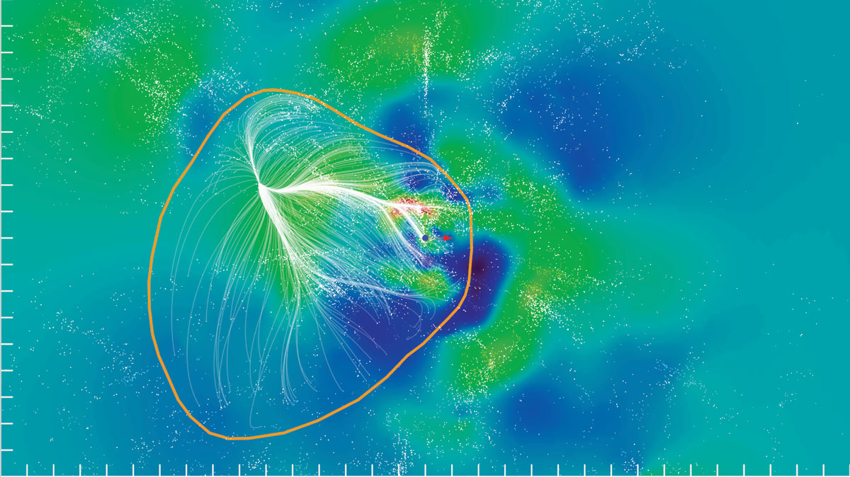
Credit: R. Brent Tully (U. Hawaii) et al., SDvision, DP, CEA/Saclay.
Unmodified image distributed by Wikimedia Commons under CC BY 4.0.
Image source ↗License ↗Provenance · JSONREADING A RECONSTRUCTION
The study inferred peculiar motions from measured distances and redshifts. Its basin definition removes the mean expansion and separates long-range flows. It does not say that every galaxy is approaching us or that the whole basin will collapse.
Streamlines describe a reconstructed velocity field. They are not observed trails across the sky or guaranteed future galaxy orbits.
Compare the published view with real telescope images above and controlled gravity experiments below. We have not re-fitted the 2014 field or imported its numerical uncertainties.
Distances, calibration, sparse sky coverage and the separation of local and external flows affect an inferred basin. Testing its stability requires numerical reconstructions and uncertainty ensembles.
Prescribed gravitational potentials in flat ΛCDM. Not an observational reconstruction or a forecast of our actual neighbourhood.
Read the assumptions ↓Arrows use the background frame, while radial diagnostics use the moving observer. Arrows show direction with a shared nonlinear length scale; use the plots or exports for velocity magnitudes. Sources follow fixed comoving paths. The observer moves freely.
Computing trajectories…
READ THE MOTION
All radial diagnostics subtract the moving observer’s velocity.
Initially collinear probes evolve in 3D; the connected curves guide the eye. This is a synthetic model profile, not a Hubble-diagram fit.
Positive total = increasing separation from the observer. Negative peculiar motion alone does not imply that separation is decreasing.
THE MODEL IS PART OF THE RESULT
A flat matter + Λ universe sets a(t). The solver evolves comoving positions x and physical peculiar velocities u. Physical positions are r = ax.
dx/dt = u/a
du/dt = g − H(a)u
da/dt = aH(a)Softened Plummer potentials represent excess mass above the homogeneous background. Their centres are fixed in comoving coordinates; mass and physical softening stay constant.
g = −Σ GM Δr / (|Δr|² + b²)³ᐟ²The sources do not react to each other or to the tracers. This is not a self-consistent N-body reconstruction.
Fourth-order Runge–Kutta uses a 0.01 Gyr step, with snapshots every 0.05 Gyr. Tests check analytic expansion, force gradients, free-particle momentum and timestep convergence.
No galaxies, initial density field, gas, dark-matter particles or Planck pixels are fitted. Parameter ranges support experiments; they are not posterior intervals.
The familiar cleaned CMB map primarily records temperature fluctuations from about 380,000 years after the Big Bang. It is not a local mass map. Its dominant motion-induced dipole is removed during processing.
The model observer’s speed above is a simulated quantity, not a measurement of the Solar System or Local Group. No CMB alignment or Planck likelihood is computed. A future test could forecast the kinetic Sunyaev–Zeldovich signal from moving gas, with explicit gas physics, masks, beams and noise.
Planck map processing ↗ · Planck kSZ analysis ↗The catalog explorer now includes all 55,877 CF4 individual distance records and counted bins from 14,140,375 selected DESI galaxy spectra. The next research stage needs cross-catalog identity matching, uncertainty and selection modeling, alternative mass reconstructions, and held-out predictions. Reproducing an attractive-looking flow does not establish the real Great Attractor’s mass or its contribution to our motion.
The existing Pantheon+ inventory has 563 nearby non-calibrator light-curve records with 446 distinct literal catalog labels. Their zHD values already contain model-based source-flow corrections; they have not been used to initialize these synthetic tracers.
Read the proposed experiment and novelty review ↗