Research note 07 · 26 October 2026 · Biswajit Jana

A link across light-years.

Physical models, instrument control, photon statistics, unresolved assumptions and experiments that could invalidate the design. A technical record, not a claim of superluminal communication.

Read the physical model Open live simulations

01 / Distance and causality

A message must cross a physical path.

Emission is an event, not an animation frame

Define emission A as the instant a new randomized bit becomes physically available at the transmitter. Define reception B as the instant its value becomes locally decodable at the distant terminal. The ordinary Minkowski causal interval is

Δs² = −c² Δt² + Δx² + Δy² + Δz².

Our sign convention is (−,+,+,+). A spacelike separation has Δs² > 0 and cannot be connected by ordinary null or timelike future-directed signals. A coordinate speed or a faster processing algorithm is not evidence of a spacelike signal. A physical curved-spacetime shortcut might still beat a specified *reference* light time without violating its actual local null cone; that weaker and more relevant transport benchmark must be distinguished from a claim of causality violation.

Two moving endpoints

In an inertial coordinate system, let Earth follow x_E(t)=E₀+v_Et and the distant terminal follow x_B(t)=B₀+v_Bt. The one-way null intercept τ satisfies:

|B(t₀+τ) − E(t₀)|² = c² τ².

After a reply-generation delay τ_p, solve a second null intercept from the then-current remote location to the then-current Earth worldline. The resulting round trip is not generally twice an instantaneous distance divided by c. The static illustrative 4.24-light-year baseline nevertheless yields about 8.48 years for an immediate reply.

Inertial 3D implementation, point-ahead and uncertainty sampling

Scope and precision

Constant-velocity worldlines are a validation baseline, not a frozen astronomical ephemeris. This code does not yet solve light propagation in a curved Solar/Galactic metric, fit Gaia astrometric covariance, model acceleration or calibrate clock transfer. Those omissions must be closed before issuing a physical Earth–Proxima pointing prescription.

02 / Optical channel and modulation

Convert joules into detected information.

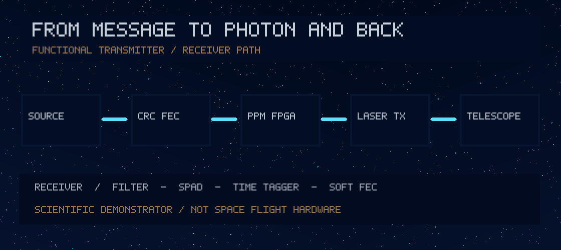
Raster systems diagram from data frame to optical telescope and receiver — Fig. 2 — Signal chain, with independent data, electrical, optical and clock subsystems.

Small-receiver diffraction benchmark

For an unobstructed circular transmitter, a receiver much smaller than the far-field diffraction spot, a monochromatic carrier and ideal acquisition, the approximate captured power fraction is

z = π D_t D_r / (2 λ R),
η_capture ≈ z²/4 − z⁴/32.

The mean detected photon rate is

Ṅ ≈ (P_t λ / hc) · η_capture · η_system.

These equations do not include telescope obscuration, imperfect wavefronts, thermal stability, optical spectral losses, pointing acquisition or detector dead time. In the live site, pointing jitter uses a separate Gaussian-equivalent approximation and must not be mistaken for an exact jitter-averaged Airy integral.

Source and regression tests

Photon statistics determine symbol decisions

With M-ary pulse-position modulation, one of M intervals contains the intended signal pulse. In an independent Poisson model, the selected slot follows Poisson(s+b) and each other slot follows Poisson(b). For b>0, the ideal hard-decision maximum-likelihood detector selects the largest observed count.

N_on ~ Poisson(s+b)
N_off ~ Poisson(b)

If background is exactly zero, the symbol error probability with random guessing after a no-photon event is

P_SER = (1 − 1/M) exp(−s).

This is an uncoded symbol error rate—not bit error rate or delivered frame throughput. The Python programme also includes seeded count simulation, 95% Wilson intervals, a simple two-axis pointing-jitter model and separate soft-decision/FEC experiments.

Reproduce the stochastic model

Where the modulation research goes next

A deployable link requires spectral stellar background estimates, detector quantum efficiency, clock recovery, acquisition, point-ahead errors, bandwidth, finite peak optical power, blocking/guard slots, CCSDS-consistent synchronization, soft information and a measured coded frame-error curve. No modulation family is assumed globally optimal; compare goodput per joule and accepted new bits per received photon across real operating conditions.

03 / Electronics: proposed engineering interfaces

A transmitter and receiver are systems, not boxes.

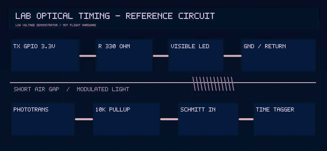
Functional low-voltage optical timing chain in original PNG format — Fig. 3 — Electronic timing demonstrator functional blocks; wiring details and test points below.

Transmitter digital and optical chain

CPUFrame + CRC

›

FPGASlot timing + FEC

›

DriverPulse-energy control

›

OpticsBeam launch

Laser module choice must be constrained by pulse width, optical average/peak power, repetition rate, optical bandwidth, heat and aging. A hardware safety interlock, watchdog and independent disable path must exist outside the user data pipeline. The pointing sensor, motor/fast steering mirror, actuator drivers and optical fiducials form a second feedback loop.

No laser driver circuitry should be treated as manufactured or electrically qualified based only on this block diagram.

Receiver optical and timing chain

OpticsPupil + filter

›

DetectorSPAD / SNSPD

›

TDCEvent tagging

›

FPGASoft decoder

The detector module's output polarity, electrical swing, timestamp granularity, dead-time distribution, dark-rate and cable propagation must be calibrated. SNSPD cryogenics and SPAD high-voltage bias/quench electronics are specialized subsystems and are deliberately excluded from the basic educational circuit.

Only packets passing the selected end-to-end integrity test count as recovered fresh information.

Low-voltage teaching experiment: optoelectronic loopback

Digital 3.3 V output → 330 Ω series resistor → visible LED → ground. Across a short enclosed air gap, place a phototransistor with emitter to receiver ground. Pull its collector/sense node up to 3.3 V with 10 kΩ and pass the signal into a compatible Schmitt-trigger input. Light should pull the sense node toward LOW; verify actual logic polarity and response delay.

I_LED ≈ (3.3 − 2.0) V / 330 Ω ≈ 3.9 mA

This current assumes a 2.0 V forward drop; select components using actual manufacturer ratings. **Do not** connect high-voltage avalanche circuitry or a high-power laser to this reference setup.

Signal / test point	Nominal interface	Required observation
TP1 — FPGA / MCU drive	3.3 V logic	Output pulse width, jitter, drive current
TP2 — LED series path	330 Ω nominal	Forward current, pulse shape, temperature
TP3 — phototransistor collector	10 kΩ pull-up, 3.3 V	Light-dependent edge latency and slew
TP4 — digital receiver	3.3 V-compatible input	Threshold crossings, timestamp jitter, BER
TP5 — common reference	Ground and timing reference	Ground loops, timing drift, noise susceptibility

04 / Quantum control

Correlated photons are not a remote keyboard.

A Bell pair gives the wrong kind of knowledge

For the Bell state |Φ⁺⟩ = (|00⟩ + |11⟩)/√2, the receiver's reduced state is one-half the identity. Alice can choose a measurement basis, but Bob's unread local probabilities do not reveal that choice.

ρ_B = Tr_A(|Φ⁺⟩⟨Φ⁺|) = I/2
P(B=0 | Alice chooses X) = 1/2
P(B=0 | Alice chooses Z) = 1/2

Two observers discover the joint pattern only after bringing their records together. Quantum teleportation has a classical communication requirement. A seeded Python null control and deliberate ordinary-leak positive control are available in the repo.

See full derivation and experiment

What could invalidate a no-signalling conclusion?

Unsynchronized time windows, post-selection, nonrandom or predictable bit choice, detector drift, a common source, hidden classical leakage or a wrongly specified causal separation can all create apparent associations. A statistically significant mutual information estimate is not proof of causal signalling.

For a purported causality-violating channel, the relevant statistic must be measured from receiver-only data recorded before any allowed causal channel could bring the fresh message, with time-correlated null surrogates and independent replication.

05 / Speculative gravitation, isolated from the hardware baseline

A spacetime shortcut needs a physical spacetime.

Suppose a proposed metric g_μν appears to connect events faster than a reference flat-space photon. That does not prove a signal outside the actual metric's light cone. The null structure, stress-energy and global causal relationships must be computed for the candidate geometry itself.

ds² = g_μν dx^μ dx^ν
G_μν + Λg_μν = (8πG/c⁴) T_μν
g_μν k^μk^ν = 0 (null rays)

Physical scrutiny includes conservation ∇_μT^μν=0, observer-dependent energy density, null/weak energy conditions where relevant, matter source dynamics, stability, chronology, and whether a usable corridor can be established in finite time. Some conditions are theory-specific; do not assume that a failure or success of one energy condition establishes the whole physical argument.

The Alcubierre warp geometry, Krasnikov-type metric, traversable wormhole and Hyperwave proposal occupy a theoretical hypothesis ledger. They are not advanced stages of the LED or photon-counting electronics. This repo has no working instrument that creates such a metric.

06 / Validation requirements

What an instrument builder would need next.

Experiment	Data to save	What must be reproducible
Timing loopback	Logic-analyser edges, clock configuration, temperature	Jitter distributions and BER as a function of pulse width
Visible optical loopback	Oscilloscope voltage/time records, light levels	Detector threshold, ambient rejection and pulse timing
Qualified photon-counter test	Time-tag stream, dark/background counts, detector datasheet	Poisson/dead-time agreement, saturation, confidence intervals
Soft PPM + FEC	Seeded messages, coded bits, slot counts and packet CRC	Symbol, bit and frame error rates versus signal photons
Moving endpoint fit	Catalog ID, epoch, position/velocity covariance	Arrival-time and pointing-error propagation with units
Candidate GR metric	Metric, inverse, Christoffels, Einstein tensor, matter model	Tensor identities, energy tests, geodesics and global causal analysis

Versioned computational record

Source Python, tests and seeded results belong in the public repository. The browser experiment can export its exact displayed parameter state and synthetic output as JSON. New physical data should include checksums, units, observation epochs, calibration lineage and data-use permission.

Open scientific programs

What has not been achieved

We have not built a space-qualified laser terminal, commissioned a single-photon receiver, frozen an astrometric Earth–Proxima solution, demonstrated measured end-to-end performance, or discovered controllable faster-than-light information transfer. This report is a foundation for those research questions.

07 / Literature and precedents

References and archived hypotheses

NASA/JPL — Deep Space Optical Communications. Laboratory and space-to-ground optical communication precedent.
CCSDS — optical physical layer and coding/synchronization standards. Refer to the actual applicable revisions when implementing compliant hardware.
Bennett et al., Physical Review Letters 70, 1895 (1993). Teleportation via quantum and classical channels.
Everett & Roman (1997). Krasnikov-type spacetime and exotic-matter considerations.
Alcubierre & Lobo (2021). Review of warp-drive spacetime physics.
Historical: Beyond the Light Cone research report. Preserve archived speculation with explicit unverified-reference markers.